Understanding Visual Feature Reliance Through the Lens of Complexity
Understanding Visual Feature Reliance through the Lens of Complexity
Authors: DIB Caren, SABA Jean Paul, WANG Romain
Article: Understanding Visual Feature Reliance through the Lens of Complexity
Table of Contents
- Introduction
- Feature Extraction via Dictionary Learning
- Detecting Complexity
- Feature Flow and Information Theory
- Experiment Summary: Exploring Feature Complexity in ResNet18
- Conclusion
1. Introduction
In this blog, we’ll take a deep dive into an insightful and thought-provoking paper authored by Thomas Fel, Louis Béthune, Andrew Kyle Lampinen, Thomas Serre, and Katherine Hermann. Their work explores the intricate mechanisms underlying how deep neural networks—specifically ResNet50—learn and represent complex features. This research, rooted in both theoretical and empirical analysis, investigates the nature of feature complexity, how features evolve over the course of training, and the computational structures that enable neural networks to generalize effectively.
The authors’ central motivation is to understand how models balance computational efficiency with representational richness. They explore why deep networks exhibit a preference for simpler features (simplicity bias), how complex features are supported within a network, and the trade-offs between redundancy, robustness, and importance of these features. V-information serves as the main complexity metric used throughout their study, offering a principled approach to quantifying how computationally accessible features are. In addition to V-information, they employ several other quantitative measures—such as importance scores derived from Gradient × Input, and redundancy and robustness metrics informed by prior work—to provide an exhaustive and structured analysis of feature learning dynamics.
Their findings have implications for model interpretability, robustness, and generalization, offering deep insights into the practical and theoretical aspects of modern deep learning systems. In this blog, we break down their study into a comprehensive guide for easier understanding.
2. Feature Extraction and Visualization
In this section, the authors explore the nature and diversity of features learned by the network. First, some general information:
Simple Features: These are easy-to-decode, frequently occurring concepts like sky, grass, and watermarks. They typically emerge early in the network and are transported through residual connections with little modification. Such features are aligned with simplicity bias and often serve as shortcuts for the model.
Medium Complexity Features: These include concepts like human-related elements, low-pixel quality detectors, and trademarks. They often represent slightly more abstract or nuanced properties and require more layers and computational effort to emerge.
Complex Features: Highly intricate concepts like insect legs, whiskers, and filament structures represent the most complex features. These require extensive processing across multiple layers and involve both the main and residual network branches to form progressively.
To be able to extract those features, the authors introduced an overcomplete dictionary as a solution to a key challenge in understanding deep neural networks: the superposition problem, where multiple features are entangled within single neurons, making it difficult to isolate and analyze individual features. In standard neural networks, activations $f_n(x)$ in the penultimate layer represent complex, often overlapping features, and the number of distinct features may far exceed the number of neurons $|A_\ell|$. To address this, the authors leveraged dictionary learning to build an overcomplete dictionary $D^*$, where $k \gg |A_\ell|$, with $k$ representing the number of atoms (or basis elements) in the dictionary. This allowed them to extract a richer set of disentangled features—up to 10,000, far more than the neuron count.
Each activation $f_n(x)$ is approximated as a linear combination of atoms from the overcomplete dictionary $D^*$, weighted by sparse coefficients $z$:
$$ f_n(x) \approx z D^* = \sum_{i=1}^k z_i d_i $$
This overcomplete setup allows for disentangling features beyond what individual neurons can represent. The dictionary $D^*$ is learned using Non-Negative Matrix Factorization (NMF), which aligns with the non-negative nature of ReLU activations. The optimization minimizes reconstruction error with non-negativity constraints:
$$ (Z, D^*) = \arg \min_{Z \ge 0, D^* \ge 0} | f_n(X) - Z D^* |_F $$
Trained on ImageNet with 58 million samples, the dictionary preserves over 99% of the model’s predictive accuracy. Once $D^*$ is fixed, features for new inputs are extracted by solving:
$$ z = \arg \min_{z \ge 0} | f_n(x) - z D^* |_F $$
The authors used MACO, an advanced feature visualization technique, to produce clearer and more realistic images of the network’s learned features. These visualizations are sorted by complexity, from the simplest to the most complex features, highlighting the increasing detail and intricacy as complexity grows.
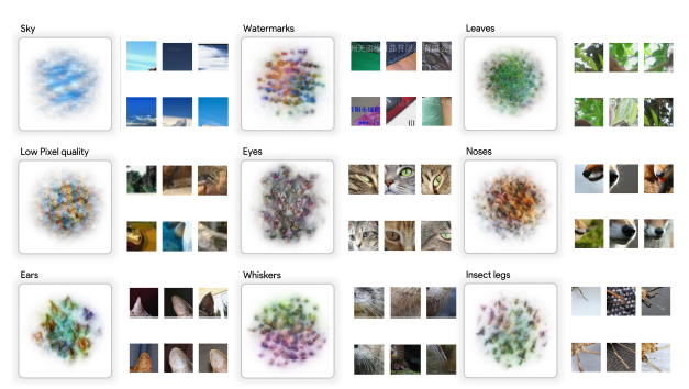 Caption: Feature Viz using MACO
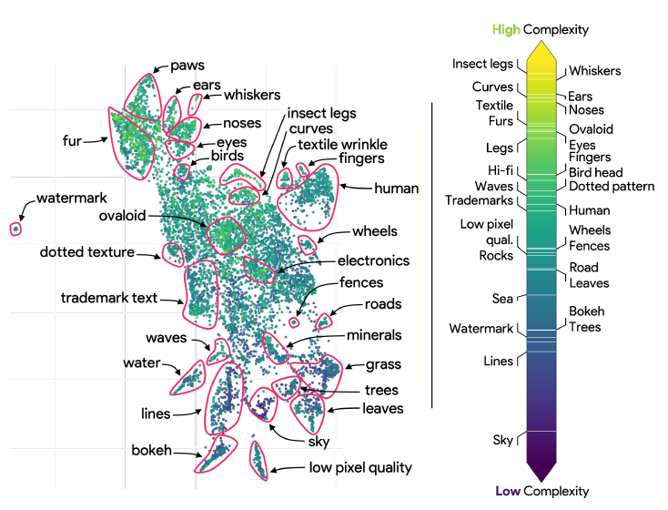 Caption: Feature complexity using UMAP
3. Detecting Complexity
The authors propose V-information as their primary metric to quantify feature complexity. They focus on a setting where the predictive family $V$ consists of linear classifiers with Gaussian posteriors. In this context, V-information measures how much information a representation $x$ provides about a feature $z$ under computational constraints. The authors derive a closed-form solution for V-information when $V$ consists of these linear Gaussian models:
$$ I_V(x \to z) = H_V(z) - H_V(z|x) $$
Here, $H_V(z)$ represents the V-entropy, which measures the uncertainty about $z$ when using the best possible predictor from the restricted family $V$. Similarly, $H_V(z|x)$ is the V-conditional entropy, which measures the remaining uncertainty about $z$ after observing $x$, again under the constraint of using predictors from $V$.
Which leads to having:
$$ 0 \le I_V(x \to z) \le \text{Var}(z) $$
Since the input data are centered and scaled, $\text{Var}(z)$ is typically close to 1. The authors define feature complexity $K(z, x)$ as the inverse of the average V-information across network layers, quantifying how difficult it is to decode a feature as it propagates through the network:
$$ K(z, x) = 1 - \frac{1}{n} \sum_{\ell=1}^{n} I_V(f_\ell(x) \to z) $$
They note that a higher $K(z, x)$ score indicates a more complex feature, harder to decode until later in the model. Empirically, they observed that $K(z, x)$ generally falls within $[0, 1]$, with 1 representing high complexity.
3.1. Relations with Redundancy
To explore the relationship between complexity and redundancy, the authors employed a redundancy measure based on Centered Kernel Alignment (CKA). In their analysis, they compared the similarity between a feature $z$ and the network activations $f_n(X)$, both before and after masking parts of the activations. A binary mask $m$ was applied to the activations, where $m \in {0,1}^{|A_\ell|}$ selects which neurons remain active (1) and which are deactivated (0). If masking neurons didn’t change the similarity much, it meant the feature was redundant, spread over many neurons. If the similarity dropped a lot, the feature was localized, relying on fewer neurons. The redundancy score was calculated as:
$$ \text{Redundancy} = \mathbb{E}_m \left[ \frac{CKA(f_n(X) \odot m, z)}{CKA(f_n(X), z)} \right] $$
Where:
$$ \text{CKA}(A, B) = \frac{|K_A K_B|_F^2}{|K_A K_A|_F \cdot |K_B K_B|_F} $$
They found that complex features are less redundant, meaning they depend on specific neurons and are more fragile.
3.2. Complexity and Robustness
The authors also investigated how feature complexity relates to robustness. They found that complex features are less robust, meaning they are more sensitive to input perturbations.
They quantified robustness by measuring the variance in a feature’s response $z(x)$ when the input $x$ was perturbed with Gaussian noise. For each input, they generated perturbed versions:
$$ \tilde{x} = x + \mathcal{N}(0, \sigma^2 I) $$
and computed the sensitivity score as the variance of $z(\tilde{x})$:
$$ \text{Sensitivity}(z) = \text{Var}(z(\tilde{x})) $$
They tested this over 100 noise samples and three noise levels $\sigma \in {0.01, 0.1, 0.5}$ across 2,000 validation images. Regardless of the metric used (variance or range), complex features consistently showed higher sensitivity to noise. This suggests complex features are more fragile and less robust compared to simpler ones.
3.3. Importance Measure
By trying to find a relation with the importance of the features, the authors focused on the penultimate layer of the network, where the extracted features $z$ are directly connected to the logits $y$. A logit is the raw output of the model before applying softmax to get class probabilities. It represents the model’s confidence for each class.
To measure how much each feature $z_i$ influences the logit $y$, the authors used the Gradient × Input method. Specifically, they computed:
$$ \Gamma(z_i) = \mathbb{E} \left[ \left| \frac{\partial y}{\partial z_i} \cdot z_i \right| \right] $$
This gives the importance score for each feature, showing how sensitive the model’s output is to changes in $z_i$. A higher score means the feature has a bigger impact on the prediction.
The authors found that simple features often have higher importance scores. These features are more directly used by the network to make decisions. On the other hand, complex features tend to have lower direct importance but may still play supporting roles in the model’s reasoning.
4. Feature Flow and Information Theory
The authors validated their hypothesis on how simple and complex features propagate through neural networks by replicating their earlier analysis with a different complexity measure. While they initially used Centered Kernel Alignment (CKA), they later confirmed their findings with V-Information, their primary complexity metric. The results were consistent: simple features showed high V-Information early and were efficiently passed through residual connections, while complex features accumulated V-Information gradually, being constructed layer by layer. This replication, done with a different ResNet50 model (Keras) and on ImageNet validation data, reinforced the idea that complex features are built progressively rather than carried intact through the network.
The authors then connected their empirical findings to concepts from algorithmic information theory, particularly Kolmogorov Complexity and Levin Complexity, to offer a theoretical foundation for their observations.
Kolmogorov Complexity measures the length of the shortest program capable of producing a given output sequence $(u_n)$ over some finite alphabet $\Sigma$:
$$ K^{(\infty)}_L(u_n) = \min_{P(n) = u_n} |P| $$
Intuitively, sequences that follow simple patterns (like $1, 2, 3, 4, …$) have low Kolmogorov complexity because they can be described by a short program. Conversely, truly random sequences have high complexity because they lack shorter descriptions. While Kolmogorov complexity captures an idealized notion of simplicity, it is not computable—there’s no general algorithm that can calculate it.
To make this concept tractable, Levin Complexity was introduced. Levin adds a penalty based on the runtime of the program, balancing the program’s length and the time it takes to run:
$$ K^{(T)}_L(u_n) = \min_{P(n) = u_n} |P| + \log |\Sigma| \cdot T(P, n) $$
Here, $T(P, n)$ represents the time the program $P$ takes to compute $u_n$. This makes it possible to compute Levin complexity through Levin Universal Search, an algorithm that runs all programs of increasing length in parallel, for one step at a time, until one halts and produces the output:
Algorithm 1 : Levin Universal Search
Input: sequence (u_n) ∈ Σ*
Output: program P minimizing K(T)_L
1: S ← ∅
2: for i ∈ N do
3:     for each program P ∈ (Σ^i ∩ L) do
4:         S ← S ∪ {P}
5:     for each P ∈ S in parallel do
6:         Run P for exactly 1 step
7:         if P halts on u_n then
8:             return P
This algorithm tends to find the simplest and fastest programs first, illustrating a simplicity bias: simpler solutions are discovered before more complex ones.
The authors argue that deep learning models exhibit a similar simplicity bias. Neural networks are effectively programs composed of weights and computations. Features that are decoded early in the network—those requiring fewer layers and simpler computation—are analogous to low Kolmogorov or Levin complexity. Features that require deeper, more complex computations align with higher complexity measures.
Their V-Information metric formalizes this intuition. It quantifies how much useful information about a feature $z$ can be extracted from an input $x$ at different layers of the network:
$$ I_V(x \rightarrow z) = H_V(z) - H_V(z | x) $$
A higher V-Information indicates a feature is easier to decode (simpler), while lower V-Information implies a feature is harder to access and thus more complex. This mirrors the relationship between program length and runtime in Kolmogorov and Levin complexities.
5. Experiment Summary: Exploring Feature Complexity in ResNet18
In this experiment, we set out to explore how complex and simple features are learned and represented in a deep convolutional neural network, specifically using ResNet18 trained on CIFAR-10. The goal was to understand feature complexity, redundancy, robustness, and importance, similar to the methods and insights presented in the research paper.
5.1. How the Code Was Structured and What Was Done
In this experiment, we worked with the CIFAR-10 dataset, which contains 60,000 color images across 10 classes, such as airplanes, cars, and birds. We split the dataset into training and validation sets and normalized the images for consistent input.
We trained a ResNet18 model from scratch on CIFAR-10 over 5 epochs using Stochastic Gradient Descent (SGD) and cross-entropy loss. The trained model achieved reasonable accuracy, making it suitable for analyzing feature representations.
After training, we extracted features from the penultimate layer and pre-pooling feature maps, which capture high-level concepts learned by the network. To further analyze these features, we applied Non-Negative Matrix Factorization (NMF), creating an overcomplete dictionary that helped disentangle individual features and overcome the issue of feature superposition.
We computed V-Information scores to measure the complexity of each feature, showing how difficult they are to decode at different layers of the network. In addition, we analyzed feature importance through logistic regression, assessed redundancy by examining feature correlations, and measured robustness by testing feature stability under noise perturbations.
Finally, we visualized the features using UMAP, projecting them into 2D space to reveal clusters based on complexity and semantic similarity. HDBSCAN clustering helped identify groups of related features, offering insights into their complexity and roles in the network’s decision-making process.
5.2. Experiment Results and Interpretation
- We plotted the features using UMAP and colored them by their complexity scores (based on V-Information).
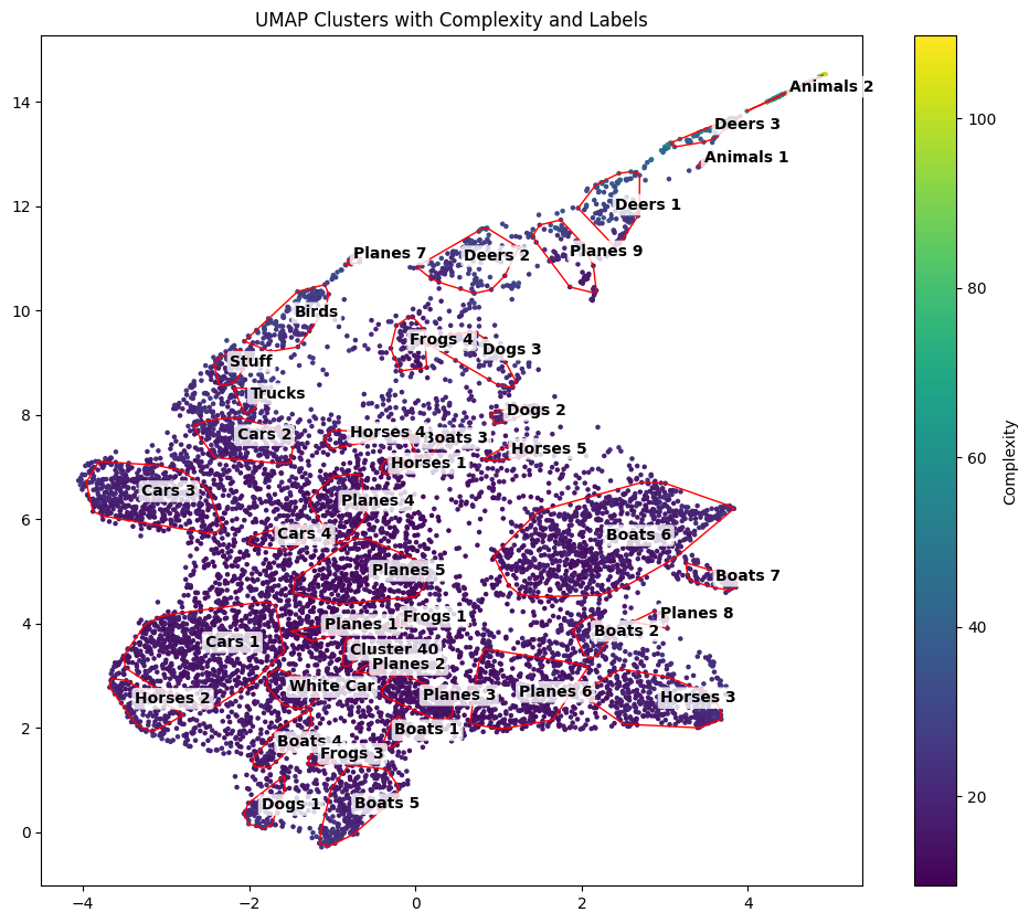 Caption: UMAP representation of the Features’ Complexity on CIFAR10 Dataset
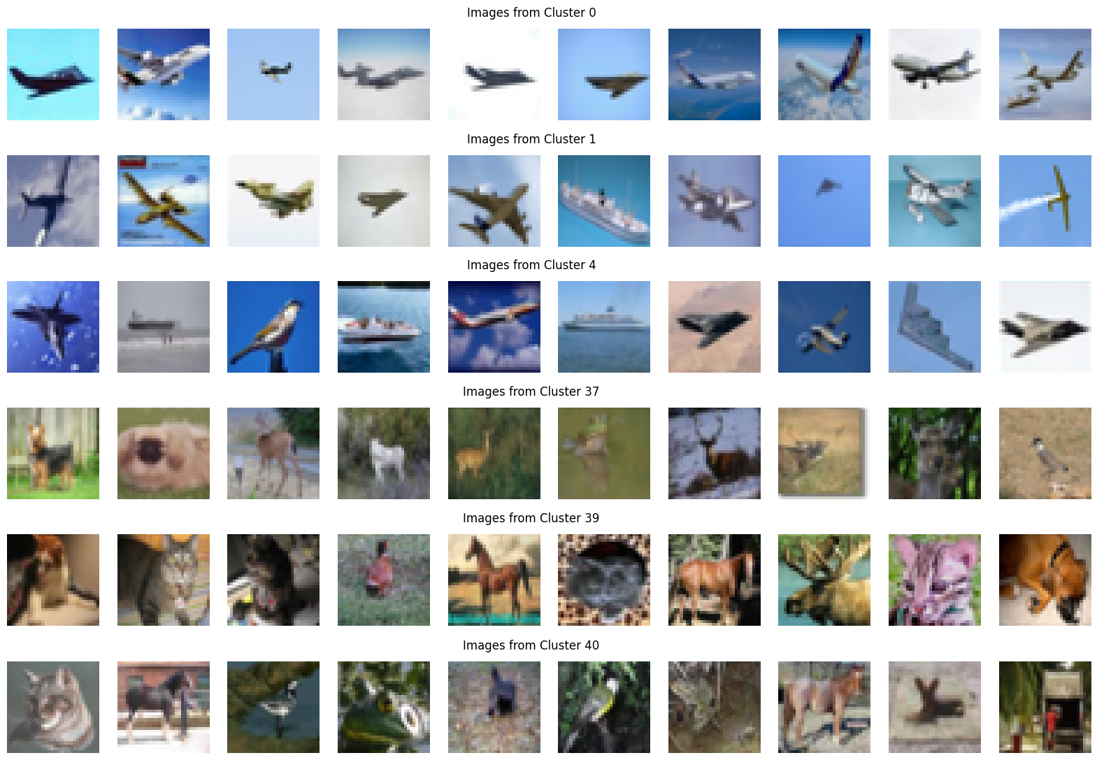 Caption: Clusters that are labeled on the UMAP Map
By applying V-Information, we clustered features based on their complexity, and visualized them using UMAP. In the second UMAP plot (Figure 2), we see clear groupings: clusters with images of planes, cars, and sky are associated with low complexity. These images are simple, with uniform regions and clear shapes, making them easier to process for the model.
In contrast, clusters labeled Animals, Deers, and Horses contain high complexity images. These images feature more visual detail, like fur, leaves, and branches, which require deeper processing and more complex feature representations.
Even with CIFAR-10’s low-resolution, the network distinguishes simple from complex features effectively. Images dominated by sky are less complex, while those with animals and rich textures show up as more complex in both the V-Information measure and the UMAP clustering.
- After analyzing the UMAP, we plotted how feature complexity relates to feature importance for classification.
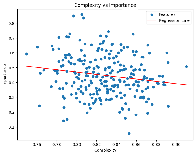
In our experiment, we plotted the relationship between feature complexity and importance to investigate how these two properties interact within the network. The scatter plot shows each feature as a blue dot, with complexity on the x-axis (measured by V-Information) and importance on the y-axis (derived from a logistic regression model trained on the features). We also added a red regression line to highlight the overall trend.
From this visualization, we found a slight negative correlation between complexity and importance. This means that simpler features, which are easier for the network to decode, tend to have higher importance in the model’s decisions. On the other hand, more complex features, which require deeper computation and are harder to extract, tend to have lower importance on their own. This result supports the findings in the paper, which argue that neural networks exhibit a simplicity bias, relying more heavily on simpler, easily accessible features during inference.
6. Conclusion
In this work, we explored the concept of feature complexity in deep neural networks, based on the paper “Understanding Visual Feature Reliance through the Lens of Complexity.” The authors introduced V-Information as a metric to measure how accessible and complex a feature is within a model. Their findings highlight a simplicity bias in networks, where simpler features are prioritized due to their ease of extraction, robustness, and importance for decision-making.
In our experiment with ResNet18 on CIFAR-10, we replicated key aspects of their methodology. Using NMF and V-Information, we analyzed feature complexity and visualized the feature space with UMAP and HDBSCAN clustering. Our results showed that simple features, such as planes and skies, clustered together and had lower complexity, while more detailed images, like animals, exhibited higher complexity. We also observed a slight negative correlation between feature complexity and importance, reinforcing the idea that networks rely more on simple features.
Overall, our experiments support the paper’s conclusions: deep networks tend to favor simple, robust features while complex ones play a secondary, less stable role in the decision process.