Measuring the Transferability of Pre-trained Models: a link with Neural Collapse Distances on Target Datasets
Authors : Marion Chadal and Julie Massé
This blog post discusses the paper “How Far Pre-trained Models Are from Neural Collapse on the Target Dataset Informs their Transferability” [1]. It provides an explanation of it so that you can understand the usefulness of measuring transferability, and a reproduction of the authors’ experiment so that you can better visualize their methodology.
Pre-trained models and fine-tuning
Pre-trained models are currently one of the most active fields in Machine Learning. They can be found in a wide range of applications, from image recognition and natural language processing to autonomous driving and medical diagnosis. These models are “pre-trained” on massive datasets, most of the time encompassing millions of examples across diverse domains. The training process leverages Deep Learning algorithms and can take weeks or even months, utilizing powerful computing resources to iteratively adjust the model’s parameters until it achieves high accuracy on the training data.
The first purpose of pre-training is to enable the model to learn a broad understanding of the world, capturing intricate patterns, relationships, and features that are not easily discernible. This extensive learning phase allows the model to develop a deep amount of knowledge, which it can then apply to more specific tasks through a process known as fine-tuning.
What is fine-tuning? It consists in adapting a general-purpose model to perform well on a specific task. This adaptation allows the model to fine-tune its learned features to better align with the nuances of the new task, enhancing its accuracy and performance. Whether it’s identifying specific types of objects in images, understanding the subtleties of natural language in a particular context, or diagnosing medical conditions from scans, fine-tuning enables pre-trained models to become specialized tools capable of tackling a wide range of applications.
Fine-tuning begins with a pre-trained model—a model that has already learned a vast array of features and patterns from a comprehensive dataset, often spanning millions of examples. This model, equipped with a deep understanding of various data representations, serves as a robust starting point. The fine-tuning process then adapts this model to a specific task by continuing the training process on a smaller, task-specific dataset. This additional training phase is typically shorter and requires significantly fewer data and computational resources than training a model from scratch, as the model already possesses a foundational knowledge base.
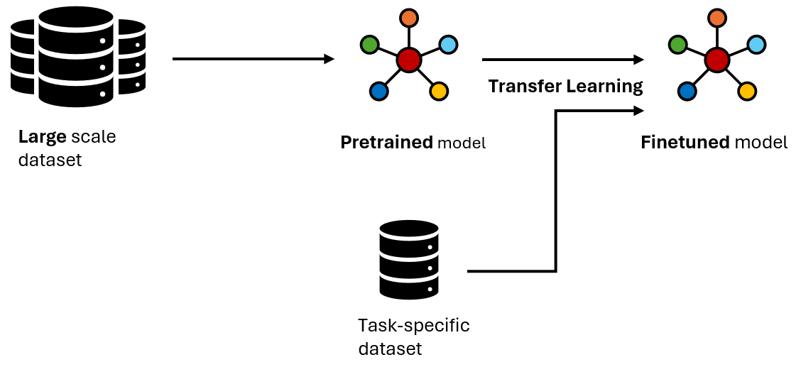
One of the key aspects of fine-tuning is its efficiency in data utilization. Since the model has already learned general features and patterns, the fine-tuning process can achieve high performance with relatively small datasets. This characteristic is particularly valuable in domains where collecting large amounts of labeled data is challenging or expensive.
Training from scratch is the complete opposite of fine-tuned pre-trained models, as it involves starting with randomly initialized parameters and requires a substantial dataset specific to the task at hand, along with considerable computational resources and time to achieve comparable performance to a fine-tuned pre-trained model. While training from scratch can be beneficial in certain scenarios where highly specialized knowledge is required or when a suitable pre-trained model is not available, the efficiency and effectiveness of leveraging pre-trained models are nowadays undeniable.
Transferability
Transferability caracterizes the ability of pre-trained models to run on downstream tasks without performing fine-tuning, but achieving comparable results. Models that exhibit high transferability are those that have learned generalizable features during pre-training—features that are not overly specific to the training data but that capture universal patterns or structures present across different datasets and domains.
Beside, transferability arises as an attempt of improvement in scalable AI, as it enables researchers and practitioners to build upon existing knowledge without reinventing the wheel for every new task. This characteristic is especially crucial in our current case where data is abundant, but labeled data is scarce or expensive to obtain. Transferable models can leverage unlabeled data from similar domains, or even entirely different domains, to achieve impressive results with minimal effort.
Moreover, the pursuit of enhancing transferability has led to innovations in model architecture, training strategies, and domain adaptation techniques. Few-shot learning for instance, where models learn from a very small amount of labeled data, and zero-shot learning, where models apply their knowledge to tasks they have not explicitly been trained on.
The concept of transferability also intersects with ethical AI development, as it encourages the use of more generalizable models that can perform equitably across diverse datasets and demographics, reducing the risk of biased or unfair outcomes.
Why measuring transferability?
Fine-tuning pre-trained models works as follows. First, you pick a downstream task, for which you have at your disposal several pre-trained models candidates. You want to compare their performances to pick the best one on test set, with the optimal fine-tuning configuration. Then, you have to fine-tune each of them. Even if the dataset to train on is smaller, thanks to fine-tuning, you have to repeat it for all your models candidates, and one does not want that, as it can quickly become computationnally expensive.
Transferability estimation arises as a solution to anticipate and avoid unnecessary fine-tuning, by ranking the performances of pre-trained models on a downstream task without any fine-tuning. Having a benchmark on the pre-trained models’ transferability would allow you to pick the relevant ones for your own downstream task.
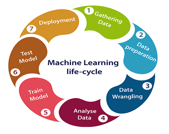
This measure is also in line with frugality in AI, which means using limited resources at every step of the Machine Learning lifecycle, while maintaining an acceptable accuracy. This frugality is especially relevant for small and medium-sized enterprises (SMEs) or startups, which may not have the vast computational resources that larger corporations possess. Transferable models democratize access to advanced AI capabilities, enabling these smaller entities to innovate and compete effectively. Frugality in AI also speaks to the broader goal of creating models that are not only powerful but also lean and efficient. Models with high transferability can achieve excellent performance across multiple tasks using significantly less data and fewer computational resources. This efficiency reduces the carbon footprint of training models and makes AI more accessible to a wider range of users and applications.
Neural Collapse
Neural Collapse happens when training beyond 0 training error, i.e training error is at 0 while pushing training loss approaching 0 even further down. Imagine training a deep neural network on a dataset for a classification task. As the training process nears its end—particularly when the model is trained to a point of perfect or near-perfect classification accuracy on the training data. Intuitively, one would expect a highly overfitted and noisy model. Instead, a remarkable simplification occurs in the way the model represents the data, as it was shown in [2]. This training approach offers better generalization performance, better robustness, and better interpretability.
Neural Collapse is characterized by three distinct proxies:
- Within-Class Variability Collapse: for any given class, the feature vectors of all samples converge to a singular point or a tightly compact cluster in the high-dimensional feature space. This collapsing effect reduces the within-class variance to near zero, meaning that all samples of a class are represented almost identically from the model’s perspective ;
- Simplex Encoded Label Interpolation (SELI) geometry: measures the gap between the features extracted by the pre-trained model and SELI geometry with the rank of the feature matrix. The higher the rank, the smaller the difference, the closer to Neural Collapse ;
- Nearest Center Classifier: ensures that the means of the collapsed points for different classes are maximally separated in the feature space.
Let’s look at this visual example of neural collapse :
Where :
- The Green Balls represent the coordinates of a simplex equiangular tight frame (ETF).
- The Red Lines represent the Final Layer Classifier. The direction of the sticks indicates the orientation of its decision boundaries, while the ball-end represents the centroid in the feature space used for classification.
- The Blue Lines represent the class means of the activations in the last hidden layer. The sticks show the variance around these means.
- The Small Blue Balls represent the last hidden layer activations. It shows how data points from each class are distributed around the class means, forming tight clusters.
Initially these elements are all scattered, but as training progresses and neuronal collapse occurs, at each epoch, they move and converged gradually as shown in the GIF.
Why choosing Neural Collapse proxies?
Let’s go back to imagining you have to perform a downstream task, and to do so you have to measure transferability between pre-trained models candidates. The three Neural Collapse proxies were previously defined, but we did not mention yet the three model’s aspects that are crucial to evaluate when choosing one:
- Generalization: through Within-Class Variability Collapse, we gain insight into a model’s ability to generalize ;
- Interpretability: the convergence toward SELI geometry not only enhances the model’s interpretability but also its alignment with optimal data representation structures. This alignment signifies a model’s capacity to distill and encode information in a way that mirrors the inherent structure of the data itself ;
- Robustness: the Nearest Center Classifier proxy underscores a model’s robustness. By ensuring that class means are well-separated, the model demonstrates resilience against noise and variability in data.
Authors in [3] demonstrate both theoretically and empirically that Neural Collapse not only generalizes to new samples from the same classes seen during training but also, and more crucially, to entirely new classes. Also, a more recent research [4] proposes a fine-tuning method based on Neural Collapse that achieves even better performance while reducing fine-tuning parameters by at least 70% !
The NCTI
Given these promising results, the authors developed a transferability estimation metric : the Neural Collapse Transferability Index (NCTI). This metric measures the proximity between the current state of a pre-trained model and its final fine-tuning stage on target, using the three neural collapse proxies defined above : Within-Class Variability Collapse, SELI geometry and Nearest Center Classifier. For each of them, a score is established : $S^m_{vc}$, $S^m_{seli}$ and $S^{m}_{ncc}$. These three scores are then grouped together using normalization to prevent one score from dominating due to different scales. The final transferability estimation metric is obtained by adding the normalized scores:
$$ S^m_{total} = S^m_{vc}(H^m) + S^m_{seli}(H^m) + S^{m}_{ncc}(H^m) $$
Where $H_m$ is the feature extracted by the $m$-th pre-trained model (after ranking a set of $M$ pre-trained models).
The higher the score $S^m_{total}$, the better the transferability of the model for target dataset.
Let’s detail the scores $S^m_{vc}$, $S^m_{seli}$ and $S^{m}_{ncc}$:
Within-Class Variability Collapse
The authors noticed that larger singular values indicate higher within-class variability because the features within the class exhibit significant variation from the mean, which is desirable for effective feature representation. But since singular value decomposition (SVD) is computationally expensive for large matrices, the nuclear norm which calculates the sum of singular values in a less expensive way was used. Additionally, as feature spaces are high dimensionnal, noise may appear and affect the calculation of variability. Therefore, instead of using the feature matrix $H^m_c$ directly, the classwise logits $Z^m_c$ are substituted to calculate the feature variability.
Thus, the score $S_{vc}$ is calculated as follow :
$$ S^m_{vc}(H^m) = - \sum_{c=1}^{C} ||Z^m_c||_* $$
Where $Z^m_c$ denotes the logits of the $c$-th class extracted by the $m$-th model.
The higher the score $S_{vc}$, the higher the within-class variability, which means that the pre-trained model is closer to the final fine-tuning stage.
SELI geometry
SELI geometry is a concept proposed in [6] as a generalized geometric structure version of the simplex equiangular tight frame (ETF). ETF is defined in the context of the phenomenon of neuronal collapse, but it is limited to balanced datasets. In contrast, SELI extends this concept to both balanced and unbalanced datasets. Difference between the two geometries is shown in the figure below :
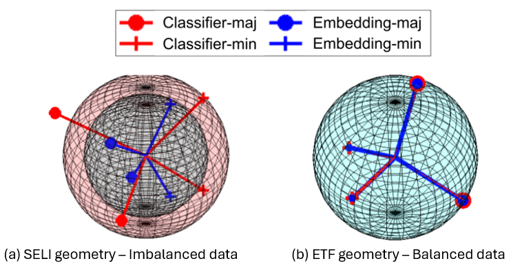
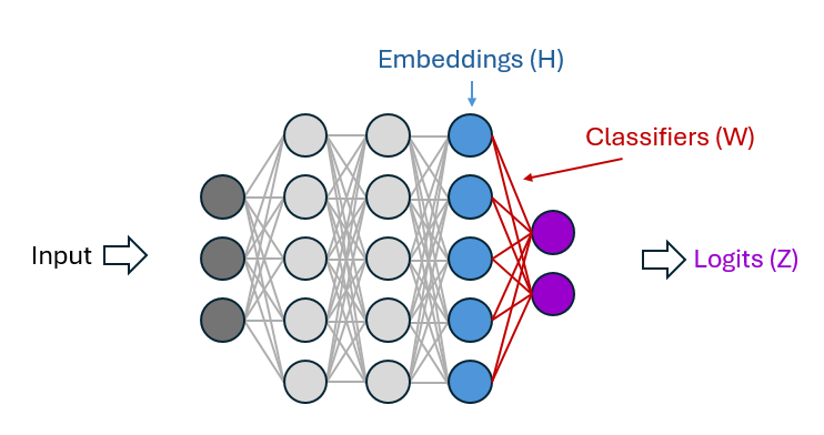
Embeddings $H$ (in blue) and classifiers $W$ (in red) follow the SELI geometry if :
$$ W^T W \alpha V \Lambda V^T, H^T H \alpha U \Lambda U^T \text{and} W^T H \alpha \hat{Z} $$
Where $\hat{Z} = V \Lambda U^T$ is the SEL matrix [6]. $U$ and $V$ denote the left and right singular vector matrix of $\hat{Z}$. $\Lambda$ represents the diagonal singular value matrix.
A method to assess the SELI geometry structure involves computing the difference between the logits $Z^m$ extracted from the pre-trained model and the optimal logits $\hat{Z}$. However, obtaining $Z^m$ directly without fine-tuning on the target dataset is time-consuming. Therefore, features $H^m$ of the model are extracted and their difference is measured to form the SELI structure. The complexity of achieving the optimal logits $\hat{Z}$ through features $H_m$ is approximated via the nuclear norm.
Thus, the score $S^m_{seli}$ is calculated as :
$$S^m_{seli}(H^m) = ||H^m||_*$$
The higher the score $S^m_{seli}$ the higher the rank of the feature matrix $H_m$, making $Z$ closer to a full rank matrix.
Nearest Center Classifier
First, the posterior probability $P(y = c|h)$ for each class $c$ is calculated using Bayes’ Rule:
$$ \log P(y = c|h) = \frac{1}{2}(h_i - \mu_c)^T \Sigma (h_j - \mu_c) + \log P(y = c) $$
Where:
- $\mu_c$ is the mean vector for class $c$.
- $\Sigma$ is the covariance matrix.
- $P(y = c)$ is the prior probability of class $c$.
- $h$ is the feature vector extracted by the pre-trained model.
Next, the softmax function is applied to obtain the normalized posterior probability $z^m_{i,c}$ for each class $c$ of the $i$-th sample:
$$ z^m_{i,c} = \frac{\exp(\log P(y = c|h^m_i))}{\Sigma ^C_{k=1} \exp(\log P(y = k|h^m_i))} $$
Where:
- $C$ is the number of classes.
- $h^m_i$ is the feature vector of the $i$-th sample extracted by the m-th pre-trained model.
Finally, the score $S^m_{ncc}$ is computed as the average of the dot product of the normalized posterior probabilities $z^m_i$ and the ground truth labels $y_i$ for all samples:
$$ S^m_{ncc}(H^m) = \frac{1}{N} \Sigma ^N_{i=1} z^m_i \cdot y_i $$
Where:
- $N$ is the number of samples.
- $y_i$ is the ground truth label of the $i$-th sample (in one-hot encoding).
The higher the score $S^{m}_{ncc}(H^m)$, the smaller the deviation to the nearest optimal centroid classifier and therefore the greater the transferability to the target dataset.
Numerical Experiment
To reproduce their experiment, the authors’ code available on a Github repository was used. A first encountered issue was the required torch and torchvision versions, which are quite old, and thus not always available to install, which was the case here. Fortunately, the most recent versions were compatible with the code. A requirements.txt file would have been welcome.
A second issue is that there are remaining personal paths in some scripts, which should be replaced by downloading paths to PyTorch source models. As a consequence, the loading method from torch should also be replaced.
Other issues considering the datasets loading remained unsolved.
After these modifications, it is possible to run the authors’ experiments on the CIFAR10 dataset for the group of supervised pre-trained models. Consisting of 60 000 32x32 colour images in 10 classes, this dataset is broadly used in benchmarks for image classification. 12 pre-trained models were ran on CIFAR10 to establish a ranking based on their performances in terms of NCTI available below.
| Model | NCTI Score |
|---|---|
| ResNet152 | 2.0 |
| ResNet101 | 1.799 |
| DenseNet201 | 1.434 |
| DenseNet169 | 1.146 |
| ResNet34 | 0.757 |
| ResNet50 | 0.709 |
| DenseNet121 | 0.655 |
| MnasNet1_0 | 0.031 |
| GoogleNet | -0.251 |
| MobileNetV2 | -0.444 |
| InceptionV3 | -0.732 |
Results show that the deepest architectures offer the best NCTI scores. The depth of a network is closely related to its ability to learn and represent complex features and patterns from the training data, which contributes to a model’s superior transferability. The different performances between ResNet and DenseNet could be attributed to the way DenseNet connects each layer to every other layer in a feed-forward fashion, which, while efficient in parameter use and reducing overfitting, may not capture as complex a feature hierarchy as ResNet. Models like MnasNet, MobileNetV2, and InceptionV3, designed for efficiency and speed with a compromise on depth, understandably score lower in transferability, as reflected by their NCTI scores.
Then, we evaluated the transferability of the supervised pre-trained models, in terms of weighted Kendall’ τ, and obtained the exact same result as the one presented in the paper: 0.843.
It was not possible for us to run the experiment on the group of self-supervised pre-trained models as the authors’ code included personal paths, and we were not able to find them online.
A Github repository with all the necessary modifications from the original code is at your disposal here.
What about source features?
Through extensive testing, authors have identified that two specific attributes related to neural collapse, observed in the source features, consistently predicted the model’s performance on new tasks. These attributes were the diversity within data categories and the compactness of category representations. Remarkably, models showing higher within-category diversity and more compact category representations in their source features tended to adapt better to new tasks. On the other hand, SELI did not consistently correlate with transferability.
Challenges
Authors did experiments on the effectiveness of each individual component in NCTI. They used the three terms individually and removed them one at a time from the full system, and it turned out that for supervised learning, the NCTI without NCC achieved the best weighted Kendall’ τ. Instead of having normalized the three NCTI components equally, it could have been interesting to tune hyperparameters. Moreover, the current implementation and validation of NCTI are confined to image classification tasks, suggesting its applicability may be limited to similar types of problems. Future work could extend the method’s applicability to a broader range of tasks beyond classification, such as detection or segmentation. Pre-trained language models could also be considered to measure their transferability based on Neural Collapse. For example, the Fair Collapse (FaCe) method [7] considers both Computer Vision and Natural Language Processing tasks, using different proxies of Neural Collapse than NCTI, and producing a slightly less good τ on the CIFAR-10 dataset (0.81).
Takeaways
Key points to remember are :
Calculating model transferability and choosing the optimal pre-trained model is important for reasons of computational cost, environmental impact, and overall performance.
The authors have developed a new metric, the Neural Collapse informed Transferability Index (NCTI), which is based on the concept of neural collapse and measures the gap between the current feature geometry and the geometry at the terminal stage after hypothetical fine-tuning on the downstream task.
The NCTI metric integrates three aspects equally: SELI geometry, within-class variability, and nearest center classifier.
This method is light to compute, enabling rapid evaluation of model transferability.
Empirical results demonstrate that the ranking of model transferability has a very strong correlation with the ground truth ranking and compares with state-of-the-art methods, highlighting its effectiveness in selecting pre-trained models for specific tasks.
In summary, the development of metrics such as NCTI is crucial for optimizing the use of pre-trained models, considering both performance and associated costs in real-world applications.
References
1. Z. Wang Y.Luo, L.Zheng, Z.Huang, M.Baktashmotlagh (2023), How far pre-trained models are from neural collapse on the target dataset informs their transferabilityWang, ICCV.
2. V. Papyan,1 , X. Y. Hanb,1 , and D.L. Donoho (2020), Prevalence of neural collapse during the terminal phase of deep learning training, National Academy of Sciences.
3. Galanti, T., György, A., & Hutter, M. (2021). On the role of neural collapse in transfer learning. arXiv preprint arXiv:2112.15121.
4. Li, X., Liu, S., Zhou, J., Lu, X., Fernandez-Granda, C., Zhu, Z., & Qu, Q. (2022). Principled and efficient transfer learning of deep models via neural collapse. arXiv preprint arXiv:2212.12206.
5. Vignesh Kothapalli, (2023). Neural Collapse: A Review on Modelling Principles and Generalization. arXiv preprint arXiv:2206.04041.
6. Christos Thrampoulidis, Ganesh R Kini, Vala Vakilian, and Tina Behnia. (2022). Imbalance trouble: Revisiting neural-collapse geometry. arXiv preprint arXiv:2208.05512.
7. Yuhe Ding, Bo Jiang, Lijun Sheng, Aihua Zheng, Jian Liang. (2023). Unleashing the power of neural collapse for transferability estimation. arXiv preprint arXiv:2310.05754v1.
Start writing here !