Statistical Minimax Rates Under Privacy
Estimating Privacy in Data Science: A Comprehensive Guide
Author: Antoine Klein Github Link
Table of Contents
- Incentives
- Introduction
- Definition
- Theory
- The case of multinomial estimation
- The case of density estimation
- Experiment
- Conclusion
- Quizz
Why do we care about privacy ?
Imagine, you’re quietly at home when the doorbell rings. You open the door and a government official appears: population census. Even though he shows you his official badge and you’d like to help him in the public interest, you find it hard to answer his questions as you go along. Indeed, the first questions about the date of your move are easy and public. On the other hand, when he asks about the number of children, marital status or your salary and what you do with it, you struggle. Not because you don’t know the answer, but because you’re faced with an ethical dilemma: transparency towards the state versus protection of personal data.
$$\text{In short, transparency goes against your privacy. }$$
This stress has major consequences: as you doubt what could happen to you with this data, but you still want to answer it, you underestimate your answers. On a wider scale, this leads to a suffrage bias and therefore a lack of knowledge of the real situation of your population. Warner [1], the first to tackle this problem from a statistical angle talks of an evasive bias and says:
“for reasons of modesty, fear of being thought bigoted, or merely a reluctance to confide secrets to strangers, respondents to surveys might prefer to be able to answer certain questions non-truthfully, or at least without the interviewer knowing their true response”
This situation presented a trusted agent, in that he wasn’t trying to harm you directly. Now imagine that you agree to give him your personal data, but that on the way home, this agent of the state is mugged and someone steals his documents. Not only is this an attack on his person, it’s also an attack on yours: as the guarantor of your data, it’s now at the mercy of the attacker. The problem here is not to have protected yourself against a malicious agent.
Admittedly, these situations are rare, but with the densification of data, their analogies are omnipresent: cookies on the Internet, cyber-attacks, datacenter crashes…One area for improvement is quite simply to better certify usage by means of cyber protection labels and leads to such a norm to achieve trust:
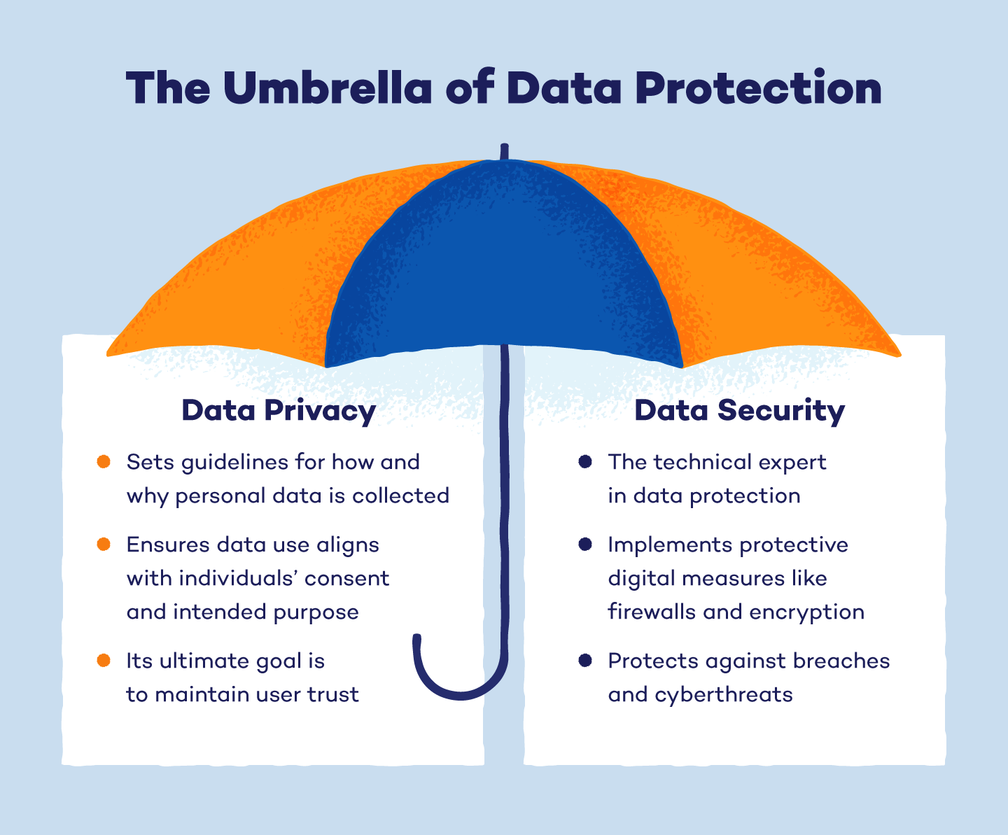
In this blog, we propose to tackle this problem from a completely different angle: how to both enable the agent to take global measures and prevent it and any subsequent malicious agents from being able to re-identify my personal data. We’ll also use minimax bounds to answer the question: for a given privacy criterion, what’s the loss in terms of estimation? (fundamental trade-offs between privacy and convergence rate)
Scientific introduction
Our blog will follow the same plan as the article that inspired it (John C. Duchi [2]),i.e. to show that response randomization achieves optimal convergence in the case of multinomial estimation, and then that this process can be generalized to any nonparametric distribution estimation. To this end, we will introduce the notion of local differential privacy as well as the minimax theory for obtaining optimal limits. All this will shed light on the trade-off between privacy and estimation rates. We will also explain algorithms to implement these optimal strategies. Finally, we will propose some experimental results.
Some key definitions
Let assume that you want to make private $X_1 , … , X_n \in X$ random variable and, as the statistician, you only observe $Z_1, . . . , Z_n ∈ Z$. The paper assumes that there exist a markov kernel that links the true ramdom variables and the observed ones as follow: $Q_i(Z_i | X_i = x)$.
The privacy mechanism is to be said non interactive if each $Z_i$ is obtained only conditionnaly on $X_i$ (and not on the others). This represents the fact that the privacy mechanism is memory less. If not, the mechnism is said to be interactive.
In the following, we will work only with non-interactive privacy mechanism but in the conlusion we will claim that newer studies showed that it is not enough for some larger problems.
$Z_i$ is said to be α-local-differentially private for the original data $X_i$ if $$sup(\frac{Q(Z | X_i = x)}{Q(Z | X_i = x’)} | x, x’ ∈ X) ≤ exp(α)$$.
An intuitive way of understanding this definition is to see that the smaller α is (the more private it is), the more difficult it is to distinguish the distribution of Z conditional on two different X data.
Theoretical results
The case of multinomial estimation
In this section, we return back to the problem of the private survey. For the statistician view, estimating a survey is estimating the parameter θ from the Bernouilli distribution $B(θ)$.
This problem is a special case of multinomial estimation, where θ is now a multidimensional parameter that is amenable to simplex probability. $∆d := (θ ∈ ℝ+ |∑θ_j = 1)$.
Theorem : Given α-local-differentially private $Z_i$, there exists some arbitrary constants $C_1$, $C_2$ such that for all $\alpha\in [0,1]$: $$C_1 min(1, \frac{1}{\sqrt{n\alpha^2}}, \frac{d}{n\alpha^2}) ≤ E[|θ_{hat} - θ|^2] ≤ C_2 min(1, \frac{d}{n\alpha^2})$$ and $$C_1 min(1,\frac{1}{\sqrt{n\alpha^2}}) ≤ E[||θ_{hat} - θ||_1] ≤ C_2 min(1,\frac{d}{\sqrt{n\alpha^2}})$$.
Recall from standard statistics: For non private independant $Z_i$ with finite variance, there exists some arbitrary constants $C_3$ such that: $$E[|θ_{hat} - θ|^2] ≤ \frac{C_3}{n}$$
In others term, providing α-local-differentially privacy causes a reduction in the effective sample size of a factor $\frac{\alpha^2}{d}$ for best situations. It thus means that the asymptotically rate of convergences remains unchanged which is a really good news !
Practical strategies
The paper deals with one of the 2 standard methods to implement such a strategy that obtains the minimax rates:
Randomized responses
The intuition of this section is the following : to not allow the statistician to retrieve your personnal data in case of Bernouilli distribution, you toss a coin. If it is heads, you say to him your reel answer, if it is tails, you say the opposite. In his point of view, as he doesn’t know what was the result of the coin, he can’t distinguish if you tell the true or not but in a large scale, he knows that he will have half correct answer, half lies so that he can retrieve information.
For the multinomial estimation now, you will generalize this procedure to the multidimensionnal setting. For each coordinate, you will tell to the statistician the reel answer with a certain probability and lies otherwise. More precisely, its leads to :
$$[Z]_j = x_j \text{ with probability } \frac{e^\frac{\alpha}{2}} {1 + e^\frac{\alpha}{2}}$$ $$[Z]_j = 1 - x_j \text{ with probability } \frac{1}{1 + e^\frac{\alpha}{2}}$$
Such a mechanism achieves α-local-differentially privacy because one can show that :
$$\frac{Q(Z = z | x)}{Q(Z = z | x’)} = e^\frac{\alpha}{2}(||z - x||_1 - ||z - x’||_1) \in [e^{-\alpha}, e^\alpha]$$ which is the criteria given above.
With the notation as $1_d=[1, 1, 1, …, 1]$ corresponds to a d-vector with each coordinate equals 1, we can also show that :
$$E[Z | x] = \frac{e^\frac{\alpha}{2} - 1}{e^\frac{\alpha}{2} + 1} * x + \frac{1}{1 + e^\frac{\alpha}{2}}1_d$$
This leads to the natural moment-estimator :
$$θ_{hat} = \frac{1}{n} ∑_{i=1}^{n} \frac{Z_i - 1_d}{1 + e^\frac{\alpha}{2}} * \frac{e^\frac{\alpha}{2} + 1}{e^\frac{\alpha}{2} - 1}$$
One can also show that it verifies :
$$E[ ||θ_{hat}- θ||_2] ≤ \frac{d}{n} * \frac{(e^\frac{\alpha}{2} + 1)^2}{(e^\frac{\alpha}{2} - 1)^2} < \frac{C_3}{nα^2}$$ which is the announced result.
Laplace Noise (beyond paper)
Instead of saying the truth with some probability, one may think of adding noise to the answer so that the statistician can’t retrieve his real answer. This is exactly the mechanism we propose to dive in and which is not covered in the paper.
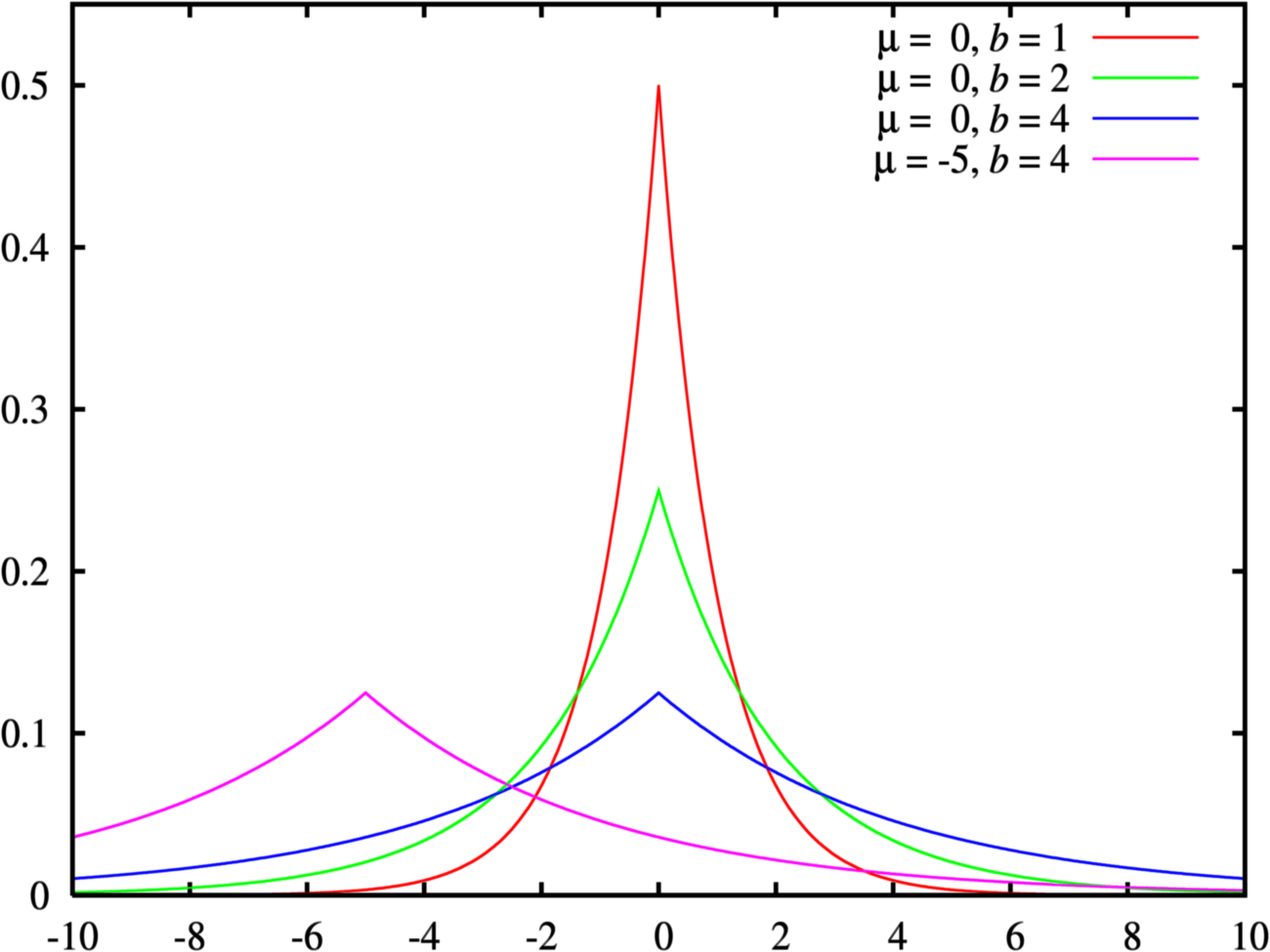
Definition: A noise is said to be a Laplace noise with parameters (μ, b) if it verifies:
$$f(x|μ, b) = \frac{1}{2b} * exp(\frac{-|x - μ|}{b})$$
A visualisation for differents parameters is given below. We can see that Laplace distribution is a shaper verson of the gaussian distribution :
The trick is to use such a noise. Let assume $X_i \in [-M,M]$ and construct the private mechanism as follow:
$$Z_i = X_i + \sigma W_i$$ where $W_i$ is drawn from a Laplace noise (0,1).
One can show that :
$$\frac{Q(Z = z | x)}{Q(Z = z | x’)} \leq e^{\frac{1}{\sigma} * |x - x’|} \leq e^{\frac{2M}{\sigma}}$$
Thus, with the choice of $\sigma = \frac{2M}{\alpha}$, it verifies α-local-differentially privacy. The proposed estimator is the following :
$$\hat{Z} = \bar{X} + \frac{2M}{\alpha} \bar{W}$$
One can show that it is an unbiaised estimator that achieves the optimal rates:
$$E[\hat{Z}] = E[X]$$
$$V[\hat{Z}] = \frac{V(X)}{n} + \frac{4M^2}{n\alpha^2} V[\bar{W}] = \frac{V(X)}{n} + \frac{8M^2}{n\alpha^2}$$
$$E[ |\hat{Z}- X|^2] \leq \frac{C_3}{n\alpha^2}.$$
This is exactly the optimal rates, quite outstanding !
The case of density estimation
One accurate question that can raise is : what about others distribution ? Is privacy more costly in general cases ? What is the trade-off ?
To answer this question, let’s precise the problem.
We want to estimate in a non-parametric way a 1D-density function f belonging to one of theses classes :
-Hölder Class (β, L): $\text{For all }x, y \in \mathbb{R} \text{ and } m \leq \beta, \quad \left| f^{(m)}(x) - f^{(m)}(y) \right| \leq L \left| x - y \right|^{\beta - m}$
-Sobolev Class: $F_{\beta}[C] := \left( f \in L^2([0, 1]) , \middle| , f = \sum_{j=1}^{\infty} \theta_j \phi_j \text{ such that } \sum_{j=1}^{\infty} j^{2\beta} \phi_j^2 \leq C^2 \right)$
In a intuitition way, those two classes express that f is smooth enough to admits Lipschitz constant to its derivative so that it doesn’t “vary” locally too much.
Theorem
Without privacy
One can show that without privacy, the minimax rate achievable for estimating a Hölder Class function is:
$$\text{MSE}(\hat{f} - f) \leq C_1 \cdot n^{-\frac{2\beta}{1+2\beta}}$$ with the estimator
$$\hat{f}(x) = \frac{1}{n} \sum_{i=1}^{n} \frac{1}{h} K\left(\frac{x - X_i}{h}\right) \text{with } h = C_2 \cdot n^{-\frac{1}{2\beta+1}}$$
In the case of d-multidimensionnal density f, the optimal rate is :
$$\text{MSE}(\hat{f} - f) \leq C_4 \cdot n^{-\frac{2\beta}{d+ 2\beta}}$$ with the estimator
$$\hat{f}(x) = \frac{1}{n} \sum_{i=1}^{n} \frac{1}{h^d} K^d\left(\frac{x-X_i}{h}\right) \quad \text{with} \quad h = C_5 \cdot n^{-\frac{1}{2\beta + d}}$$
This illustrates once again the curse of dimensionnality.
With privacy
Let assume that f bellongs to one of the two classes with β as smoothness parameter.
Then, the optimal α-local-differentially private optimal rate is :
$$\text{MSE}(\hat{f} - f) \leq C_1 \cdot (n\alpha^2)^{-\frac{2\beta}{2\beta+2}}.$$
One may observe two pessimistic news:
-The rate is affected by a factor of $\alpha^2$ as for the multinomial estimation
-More damageable: the rate is slower in term of n unlike the previous problem which make privacy in this case more costly.
Practical strategies
Eventhough this rate is pessimistic and proves that privacy comes at a cost, it remains to illustrates how can we achieves this best but not great rate. For this end, once again, two strategies are possible.
Randomized responses
This is the strategy illustrated in the paper and consists of sampling for each coordinate according the realisation of a Bernouilli variable with the correct probability as function of α.
As it is not the most comprehensive and straightforward method, we prefer to dive in depth into the second one; uncovered in the paper.
Laplace Noise (beyond paper)
Let assume that $X_i \in [0,M]$ almost surely. We note $G_j = [\frac{j-1}{K},\quad \frac{j}{K}]$ the bin of length $\frac{1}{K}$.
We consider the histogramm estimator: $$\hat{f}(x) = \frac{K}{n} \sum_{j=1}^{K} \sum_{i=1}^{n} 1_{X_i \in G_j} \cdot 1_{x \in G_j}.$$
We now construct the private mechanism as follow:
$$Z_i = \left[1_{X_i \in G_1} + \frac{2}{\alpha} W_1, \ldots, 1_{X_i \in G_K} + \frac{2}{\alpha} W_K\right]$$
In an intuitive way, we add a Laplace noise realisation for each bin.
This guarantees α-local-differentially privacy as : $$\frac{Q(Z = z | x)}{Q(Z = z | x’)} \leq \exp\left(\frac{\alpha}{2} \sum_{j=1}^{K} |1_{x \in G_j} - 1_{x’ \in G_j}| \right) \leq \exp\left(\frac{\alpha}{2} \cdot 2\right).$$
This leads to the α-local-differentially private estimator :
$$f_{\text{private_estimate}} = \hat{f} + \frac{2K}{n\alpha} \sum_{j=1}^{K} W_j$$
The biais is the same as the unprivate case as :
$$E[f_{\text{private_estimate}}] = E[\hat{f}] + 0 .$$
One may prove that if f bellongs to the β-Hölder Class:
$$Biais(f_{\text{private_estimate}}, f) \leq C_1 * K^{-\beta}$$
Meanwhile, $$V[f_{\text{private_estimate}}] \leq \frac{C_2}{n} + \frac{4K^2}{\alpha^2} \frac{V[W]}{n}$$, such that in total :
$$\text{MSE}(f_{\text{private_estimate}} - f) \leq C_1 K^{-2\beta} + \frac{C_2}{n} + \frac{C_3 K^2}{n\alpha^2}.$$
Minimizing over K (hyperparameters) leads to : $K = C_4 \cdot (n\alpha^2)^{-\frac{1}{2\beta+2}}$ and thus to:
$$\text{MSE}(f_{\text{private_estimate}} - f) \leq C_5 \cdot (n\alpha^2)^{-\frac{2\beta}{2\beta + 2}}$$, which is the expected bound.
Experiment: Illustration of the Minimax privacy rate
Overview
The aim of this section is to provide illustrations of the theoretical results set out above. Emphasis is placed on convergence results, with empirical confirmation of the latter.
For the sake of reproducibility and transparency, the source code can be found in the notebook at this: Github link.
Methodology
- Data Preparation: Rather than working with real datasets, we decide to work with simulated data, as this allows us to maintain control over all aspects.
More precisely, we give ourselves $n=1000$ samples of the normal distribution $N(100,1)$ on which we add a Laplace noise $L(0,\alpha).$
As for the different alpha values, we iterate through them: $[0.2, 0.3, 0.5, 0.7]$
Privacy Metric Calculation: We will look at the use case of estimating the mean of a distribution.
Evaluation: The results will be compared in terms of Mean Square Error (MSE).
Results
In terms of the observed distribution (private because subject to Laplace noise) relative to the true data, we obtain the following figure:
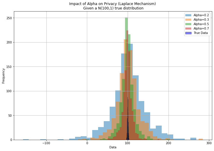
As expected, the greater the desired privacy (low $\alpha$), the more spread out the distribution of observed data.
When it comes to estimating the true average from private data, we obtain the following figure:
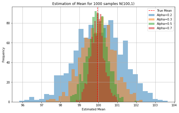
This figure illustrates two major points:
-The first is that whatever the level of privacy, we have an unbiased estimator of the mean. It’s a beautiful property, empirically verified !
-The second is that, unfortunately, the greater the privacy (low alpha), the greater the variance of this estimator.
We recall our main theorem demonstrated above Previous theorem :
Theorem : Given α-local-differentially private $Z_i$, there exists some arbitrary constants $C_1$, $C_2$ such that for all $\alpha\in [0,1]$:
$$C_1 min(1, \frac{1}{\sqrt{n\alpha^2}}, \frac{d}{n\alpha^2}) ≤ E[|θ_{hat} - θ|^2] ≤ C_2 min(1, \frac{d}{n\alpha^2})$$
We now want to compare the theoretical optimal rate with empirical results. To do this, we distinguish two situations:
-The first is with fixed alpha, and determines the MSE as a function of the number of samples n. This leads to these empirical results:
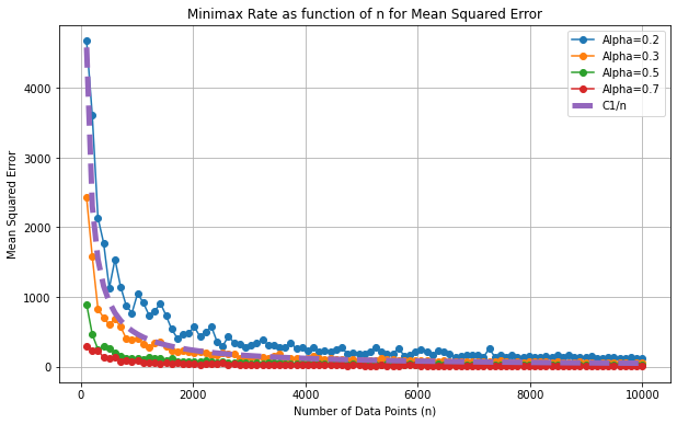
The dotted line represents the regime of the theoretical bound of the form $n \rightarrow \frac{C1}{n}$ . This is the shape of the empirical curves!
-The second has a fixed n and determines the MSE as a function of alpha. This leads to these empirical results:
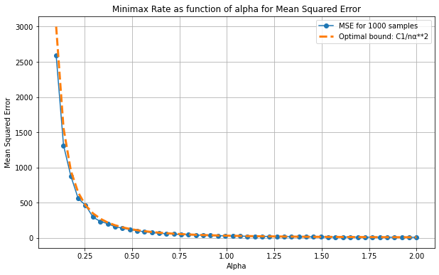
The dotted line represents the regime of the theoretical bound of the form $\alpha \rightarrow \frac{C1}{\alpha^2}$ . This is once again the shape of the empirical curves quite surprisingly!
Conclusion
From a problem rooted in an ethical dilemma (privacy versus completeness and transparency), we have looked at the cost of guaranteeing one at the expense of the other, to better sketch out desirable situations.
This has enabled us to develop theoretical results in terms of minimax rates. There is indeed a trade-off between these criteria, which is even more costly in the case of non-parametric density estimation.
Finally, we have compared these theoretical limits with empirical results, which confirm the conformity of the statements.
The aim of all this work is to disseminate this important yet under-exploited notion: privacy. To this end, we invite the reader to take the following quiz to ensure his or her understanding.
Quizz
To test yourself abour privacy:
Annexes
References
- Warner SL. Randomized response: a survey technique for eliminating evasive answer bias. J Am Stat Assoc. 1965 Mar;60(309):63-6. PMID: 12261830.
- John C. Duchi, Michael I. Jordan, and Martin Wainwright. Local Privacy and Minimax Bounds: Sharp Rates for Probability Estimation. Advances in Neural Information Processing Systems (2013)
- Dwork, C., & Roth, A. (2014). The algorithmic foundations of differential privacy. Foundations and Trends® in Theoretical Computer Science, 9(3-4), 211-407.
- Narayanan, A., & Shmatikov, V. (2008). Robust de-anonymization of large sparse datasets. In Security and Privacy, 2008. SP 2008. IEEE Symposium on (pp. 111-125). IEEE.