Do Perceptually Aligned Gradients imply Robustness?
Robustness and Perceptually Aligned Gradients : does the converse stand ?
Author: Yohann Zerbib
Table of Contents
- Introduction
- Adversarial Attacks
- Perceptually Aligned Gradients
- Experiment
- To go further
- Conclusion
- References
This is a blog post about the paper Do Perceptually Aligned Gradients Imply Robustness?, published by R. Ganz et al. in 2023 and available here.
Introduction
In the context of image recognition in Machine Learning, one could quickly realize that building robust models is crucial. Having failures could potentially lead to worrying outcomes and it is part of the design to aim to implement models that would be prevented against adversarials attacks, that will be explained. At some point, when reaching models that are robust, it somehow occurs that small variations made are easily interpretable by humans, something which is not common in current ML models such as this one. Having noticed this phenomenon, the authors of the paper would try to verify the opposite assumption. By building models that verify this idea of alignment with human perception, do we create robust models ?
Adversarial attacks
But before explaining the article, it could be relevant to explain briefly what are adversarial attacks and how it led to the design of robustness.
Adversarial attacks refer to a class of techniques in machine learning where intentionally crafted input data is used to deceive or mislead a model, leading it to make incorrect predictions or classifications. These attacks exploit vulnerabilities in the model’s decision-making process, taking advantage of the model’s sensitivity to small changes in input data that might be imperceptible to humans. They are most prominently associated with deep learning models, particularly neural networks, due to their high capacity and ability to learn complex patterns.
Concretly, in a theoretical framework, the usual example is to make a model classify an image of a cat as a dog or another animal, without any way for the human to notice it. However, consequences can be more dreadful in real life as one could consider what would happen if an autonomous vehicles missclassified a stop sign as speed limit sign.
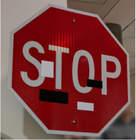
(Eykholt et al. [1])
Now, let’s dive a bit deeper to understand how these errors happen. Several points can be highlighted, such as the level of linearity of Neural Networks, but one acknowledged moot point dwells on the use of Loss function in Deep Learning methods. Indeed, especially when considering datasets of pictures, there are many directions where the loss is steep. It would mean that it can be highly delicate to propose a good minimization of the loss. Moreover, the main idea for our problem is that a small change of the input can cause abrupt shifts in the decision process of our model. This effect increases with the dimensionnality (quality of pictures…) and therefore will still be relevant with time.
The basic modelisation of an attack would be the following. Let’s consider :
- a model $f\ :\ \mathcal{X} \ \rightarrow \ \mathcal{Y}$
- the input to pertub : $x \in \mathcal{X}$
- a potential target label : $t \in \mathcal{Y}$
- a small perturbation : $\eta$
Then, mathematically, the attacker would try to have something that verifies $f(x + \eta) = t$ (or any other label than $f(x)$ for an untargeted attack).
Now, as one can imagine, it is possible to compute attacking models related to this framework. Let’s understand two well-knowns algorithms that follow this goal.
Fast Gradient Sign Method (FGSM) :
This method can be targeted or untargeted. Let’s study the targeted one. The algorithm is the following [3]: One compute the perturbation $\eta \ =\ \epsilon \ \cdotp \ sign( \ \nabla x\ L( x,\ t) \ )$ where $\epsilon$ is the perturbation size. Then, one would have $x’\ =\ x\ −\ \eta $ such that we remain espilon close from $x$ and that $f(x’) = t$. The perturbation has to remain small to ensure it will be undetected by human’s perception.
But, at this point, one question arises : how can we be sure that $x’$ is still close to $x$? How can we be sure that we have $||x\ −\ x’||_{p} \ \leq \ \epsilon $ where p is a particular norm? To answer this question, norms are introduced and two important ones, used in the article are the following.
$L_{2 }$ norm : This norm captures the global quantity of changes. It is the euclidean distance.
$L_{\infty }$ : This norm captures the maximum change in the vector.
So, we have several ways to have a level of control over the changed features.
Now that the first intuition for attack is understood, one should take a rapid look at PGD (Projected Gradient Descent) [4], which will be used for the results of this blog. Other more complex methods exist (AutoAttack), and they are taken into account by the authors but they will not be explained here.
The algorithm starts with an initial perturbation. At each iteration, the algorithm takes a step in the direction of the gradient of the loss function with respect to the input. The gradient is calculated using backpropagation, and represents the direction of steepest ascent in the loss function. However, since we’re trying to reach a specific target, we actually want to move in the opposite direction, so we multiply the gradient by -1 (it is a maximization). The step size is proportional to the norm of the gradient, so we don’t overshoot or undershoot our target. After taking a step, the perturbation is projected back onto the allowed range, which is defined by the epsilon parameter. This is done by calculating the difference between the current input and the original input, and then scaling this difference so that it falls within the allowed range. This process is repeated for a certain number of iterations. (In this version of the algorithm, there is no control that it will truly be missclassified : one has to set an improtant enough number of iterations).
However, our role here is not to learn how to create the best attacks, but more to learn how to defend them! And suprisingly, what has been shown is that the best way to achieve this goal is to have a training that includes adversarial attacks. Then, it all comes down to this optimization problem :
$\min_{\theta }$ $\mathbb{E}_{(x, y)} $ [A] where
A = $(\max_{\eta \leqslant \epsilon }$ $L( f_{\theta}( x\ +\ \eta ) ,\ y))$
This is more or less an optimization problem to solve with $\theta$ the parameters to be learnt and where each training sample has a perturbation (an attack). It is linked with adversarial accuracy. We can train a model to be more robust, but chances are it will be less performant. It is up to the trainer to choose the best trade-off on a model.
Perceptually Aligned gradients
Finally, it is possible to dive more in the subject of the article. Training models as presented before, with a particular care to robustness empirically leads to have perceptually aligned gradients. Here, one should understand “gradient” as the mathematical concept, a vector which points to the direction of the greatest increase of its function. In other words, Perceptually Aligned Gradients correspond to a property, a byproduct of robust models, where the gradients are meaningful to humans. When the input image is slightly modified, the corresponding gradient directions reflect the changes that are perceptually relevant. In other words, the gradients make sense from a human perspective.
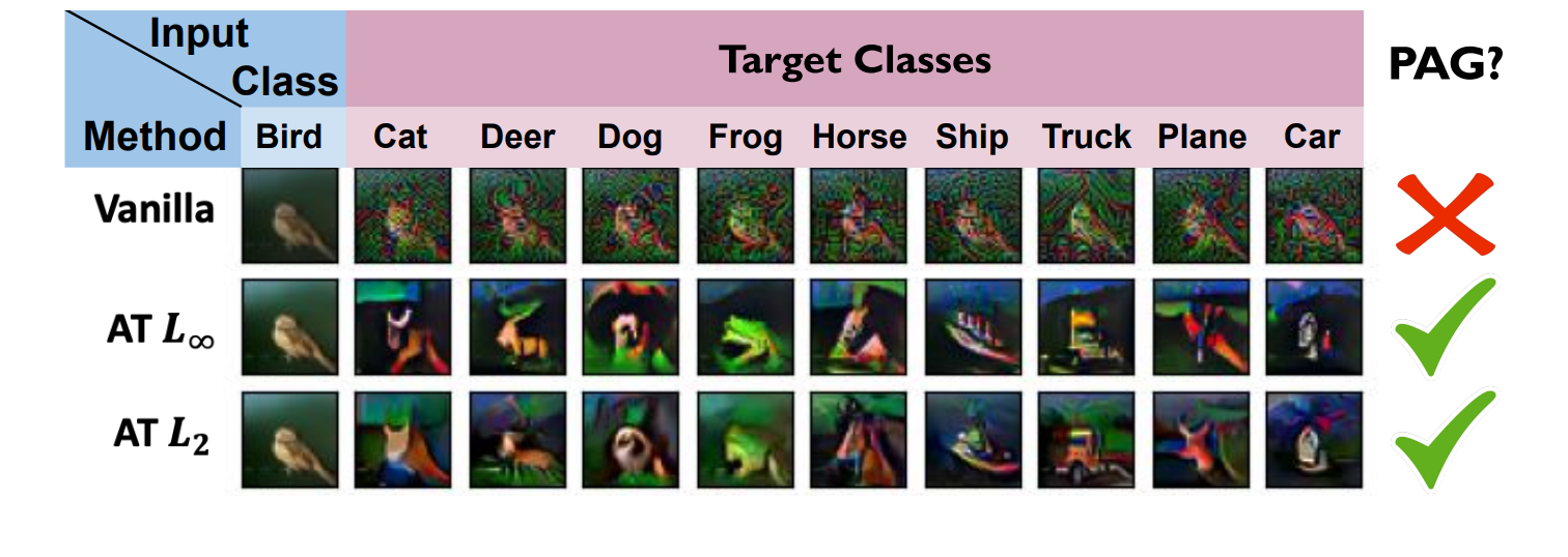
Here an example given by the author on the CIFAR dataset ([2], Ganz et al.). The intuition is that for models other than the vanilla one, the target class representative of the adversarial examples contains an information about the new class. For example, going from a bird to a frog will get the image much more green and in the shape of the frog. It looks like a ghost information.
Now, is it a Bidirectional Connection ? Let’s try to have some hints about it.
The first step to tackle this issue is to create those Perceptually Aligned Gradients without adversarial training.
Then, it is shown that models with aligneds gradients can be considered as robust.
Finally, a demonstration of the improvement of robustness through the increase of gradient alignment is proposed.
1. Algorithm of the Model
To disentangle the creation of PAG with the usual robust training, a new method is developed. It relies on two elements.
the classical cross-entropy loss from the usual categorization problem framework,
an auxiliary loss on the input-gradients, differentiable.
Then, our global loss function would look like this :
$L( x,\ y) \ =LCE\ ( f_{\theta }( x) ,\ y) \ + \lambda\sum_{y_{t} =1}^{C}L_{cos}( \nabla_{x}f_{\theta }(x)_{y_t},\ g( x,\ y_t))$
It is similar to training with a regularization part ($\lambda$ would control the power of the regularization). $L_{cos}$ is the cosine similarity loss (it gives information on the similarity of the arguments).
This does not use robust model of any sort, on the hypothesis that we have ground-true PAG in the input. This is a strong hypothesis, and it is crucial to choose well those grounds-truth. Indeed, a lack of rigor here could lead to a bias. If the ground-truth was obtained through adversarial training previously, then this new approach would only be an equivalent of adversarial training, and that is something that must be avoided. This hypotesis will be studied just a bit later.
After minimizing the loss, the model is tested through adversarial attacks (here, targeted PGD on the test set) to see if there is clearly PAG and if the adversarial accuracy is good.
2. Creation of Perceptually Aligned Gradients
As we have seen in the formula just above, it is mandatory to have a ground-truth perceptually gradient $g( x,\ y_t)$ for each training image and for each target class. However, finding those gradients are difficult and they are approximated. Firstly, let’s consider the heuristics to understand what happens.
With this objective in mind, we follow a straightforward assumption: the gradient $g( x,\ y_t)$ ought to align with the overall direction of images belonging to the target class $y_t$. Hence, when provided with a target class representative, $r_{y_t}$, we establish the gradient to direct away from the current image and towards the representative. In other words, $g( x,\ y_t) = r_{y_t} - x$
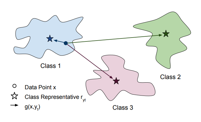
To implement this heuristic, three setups are provided.
$\textbf{One Image (OI):}$ Choose an arbitrary training set image with label $y_t$, and set $r_{y_t}$ to be that image as a global destination for $y_t$-targeted gradients.
$\textbf{Class Mean (CM):}$ Set $r_{y_t}$ to be the mean of all the training images with label $y_t$. This mean can be multiplied by a constant to obtain an image-like norm.
$\textbf{Nearest Neighbor (NN):}$ For each image $x$ and each target class$\ y_{t} \ \in \ {{1,\ 2\ .\ .\ .\ ,\ C}}$, we set the class representative $r_{y_t}(x)$ (now dependent on the image) to be the image’s nearest neighbor amongst a limited set of samples from class $y_t$, using L2 distance in the pixel space. More formally, we define $r( x,\ y_{t}) \ \ =\ \underset{ \begin{array}{l} \widehat{x\ } \in \ D_{y_{t}} \ s.t.\ \hat{x} =x \end{array}}{\arg\min} ||x\ −\ \hat{x} ||_{2}{}$
where $ D_{y_{t}}$ is the set of sample images with class $y_t$.
Now, the more theoretical approach is provided thanks to score-based gradients. Authors have used Denoising Diffusion Probabilistic Models (DDPMs), to generate approximations of PAG.
Let’s consider noisy versions of an image $x$, noted as $({x_{t}})_{t=1}^{T}$ and their distribution
$(p_t({x_{t})})_{t=1}^{T}$.
An iterative process is employed for sampling, which begins from Gaussian noise and proceeds along the direction of the score function, defined as $\nabla_{x_t} \log p(x_t)$ and approximated by a neural network. It is suggested to incorporate class information into these networks, allowing them to model a class-dependent score function $\nabla_{x_t} \log p(x_t|y)$. We identify a resemblance between the class-dependent score function and classification loss gradients with respect to the input image, leading us to propose that gradients derived from DDPM can serve as an enhanced source for perceptually aligned gradients. We would have (one term disappears with the gradient w.r.t the input image) using Bayes’ formula.
\begin{equation} \nabla_{x_t} \log p(x_t|y) = \nabla_{x_t} \log p(y|x_t) + \nabla_{x_t} \log p(x_t), \end{equation}
which results in
\begin{equation} \nabla_{x_t} \log p(y|x_t) = \nabla_{x_t} \log p(x_t|y) - \nabla_{x_t} \log p(x_t). \end{equation}
This formulation introduces a new application of diffusion models – a systematic approach to estimate the appropriate gradients for the expression $\log p(y|x_t)$. However, classification networks operate on noise-free images ($x$) rather than noisy ones ($x_t$). To link classifier input-gradients with DDPMs, we assume that $\log p(y|x) \approx log p(y|x_t)$, for certain noise levels $t$. Consequently, the desired estimation of “ground-truth” classifier input-gradients can be acquired by subtracting an unconditional score function from a class-conditional one. The selection of $t$ when distilling gradients through this method presents a tradeoff – excessively large values yield gradients unrelated to the input image (too noisy), while excessively small values produce perceptually insignificant ones (in low noise levels, the conditional and unconditional scores are nearly identical). Therefore, we choose $t$ to be of moderate values, generating both perceptually and image-relevant gradients. We denote this method as Score-Based Gradients (SBG).
To understand a bit more how it works, one has to consider that the variations of the noise from every $x_t$ can be controlled. Indeed, each different iteration takes the direction of the distribution $\log p(x_t)$ (with stochasticity). In other terms, it takes the direction of our score function that can be estimated thanks to Neural Networks. That’s how you obtain your set of ground-truth gradients related to the input images.
At this point, we have four ways to approximate ground-truth gradients. (Three heuristics and a more theoretical one). The experiments presented here will use the NN approach that are very intuitive. What was favoured for real datasets was the score-based approach.
Experiment
Now, let’s experiment a bit. In this article, to understand what is happening, we will play a bit with the toy dataset. A 2 dimensional synthetic dataset is built. It contains 6000 samples of 2 classes. Every sample is on the line of equation $x_2 -2x_1=0$. Finally, each class contains three mods (1000 samples per mode) drawn from a Gaussian distribution. The idea is to observe manifolds as decision boundaries. Background of the plan will be colored according to the predicted class. Evaluation will be made on a test set.
The code is available at this link.
To this prediction task, a simple 2 layers MLP with ReLU is used. Two training are made with the same seed. The first is based on the usual cross-entropy loss whereas the second is made on the explained new loss.
As expected, 100% accuracy is obtained for this very simple task for both models on the test set. However, what about predicting adversarial examples ?
Let’s first try it out with a targeted $L2$ PGD. Vanilla is only correct for 35 out of 600 samples, whereas this new approach obtains 583 out of 600. How can this be explained ? One should observe the decision boundaries.
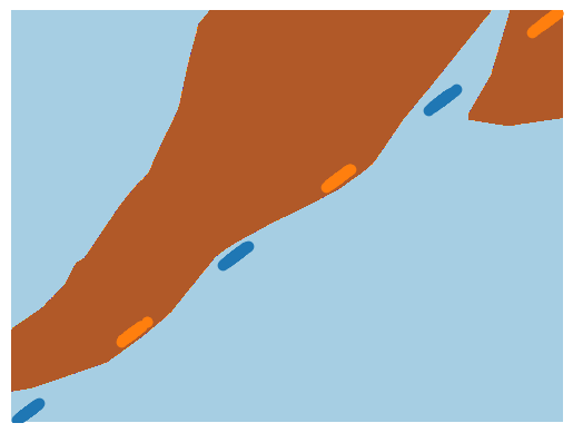
This is what is obtained for the regular neural network with cross-entropy Loss.
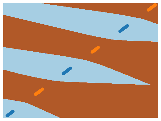
Here is the result obtained for the particular neural network with the new loss.
What one should notice is the decision boundaries. The vanilla neural network provides manifolds that really stick to the data points. Going just a bit further can on the graph really can create a shift in the prediction. And that is what is happening with a targeted pgd, where there is only a small variation (semantically invisible).
However, in the case of the PAG Neural Network, one can observe that around a mode of points, there is a much greater margin of the same class. This can be understood from the setup to create perceptually aligned gradients. Indeed, as we have seen, a target class was set based on a nearest neighbour approach, and the gradient point away from the current image and towards the class representative. Only then the cosine similarity between this gradient and the ground-truth approximated one from DDPMs.
Another possibility would be to see the impact of the size of the perturbation on the performance. Indeed, here, the given results corresponded to an epsilon value of 15. Increasing it decreases the accuracy to 75%. However, at a certain point, an augmentation of epsilon will not change anything anymore, probably because of a normalizing step in the targeted PGD algorithm.
To go further
What’s next ? Testing the hypothesis on real datasets. Among them, CIFAR-10, STL (higher resolution) and CIFAR-100 (higher number of classes). The architecture to achieve those tasks are classical (Resnet-18, ViT). Here are the main results that can be highlighted.
PAG approach is often similar and sometimes outperforms adversarially training approach. Score-based gradient seems to be the most accurate ground-truth approximation setup. It is also more notable for the ViT architecture. It also globally performs well on STL and CIFAR-100 (sometimes even better than adversarially training).
But, the question is not yet answered : Do Perceptually Aligned Gradients imply Robustness?
And that’s where the regularization aspect of the loss is very useful. One can make variation over the hyperparameter $\lambda$ to see what brings a bigger focus on the PAG loss. The authors have done it and are summarized with this table.
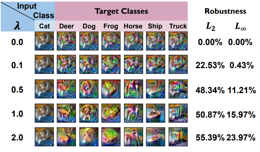
As one can see, the robustness increases with the increase of the regularization hyperparameter. The more the ghost features of the target class are visible (even if it not always comprehensible), the more the model is robust.
So, it seems that yes, models with PAG would be more robust.
Conclusion
To draw a conclusion, this paper has empirically shown that PAG lead to more robustness in models. It was also mentionned that it could potentially be combined with Adversarially Training to gain more robustness, and there are probably some experiments and tests that could optimize that. The performance are also good and can be seen as an alternative, potentially not too costly. Sometimes it ouperforms Adversarially Training and it would be up to the user to decide which framework to employ for creating robust models. Finally, approximating ground-truth PAG needs additionnal research and discussion as even if the results tend to favour Score-Based Gradients, it happens that heuristics function better and there are potentially other approaches that have yet to be discovered. One should shed light on the fact that the diffusion models used need to be trained, and the training time gained over adversarially training is not as significant as with other heuristics if we consider this aspect.
References
EYKHOLT, Kevin, EVTIMOV, Ivan, FERNANDES, Earlence, et al. Robust physical-world attacks on deep learning visual classification. In : Proceedings of the IEEE conference on computer vision and pattern recognition. 2018. p. 1625-1634.
Ganz, R., Kawar, B., & Elad, M. (2023, July). Do perceptually aligned gradients imply robustness?. In International Conference on Machine Learning (pp. 10628-10648). PMLR.
Goodfellow, I. J., Shlens, J., & Szegedy, C. (2014). Explaining and harnessing adversarial examples. arXiv preprint arXiv:1412.6572.
Madry, A., Makelov, A., Schmidt, L., Tsipras, D., & Vladu, A. (2017). Towards deep learning models resistant to adversarial attacks. arXiv preprint arXiv:1706.06083.