RobustAI_RegMixup
RegMixup : Regularizer for robust AI
Improve accuracy and Out-of-Distribution RobustnessAuthors: Marius Ortega, Ly An CHHAY
Paper : RegMixup by Francesco Pinto, Harry Yang, Ser-Nam Lim, Philip H.S. Torr, Puneet K. Dokania
Table of Contents
Abstract
Authors: Marius Ortega, Ly An CHHAY
Paper : RegMixup by Francesco Pinto, Harry Yang, Ser-Nam Lim, Philip H.S. Torr, Puneet K. Dokania
Table of Contents
Abstract
In this blog post, we will present the paper “RegMixup: Regularizer for robust AI” by Francesco Pinto, Harry Yang, Ser-Nam Lim, Philip H.S. Torr, Puneet K. Dokania. This paper introduces a new regularizer called RegMixup, which is designed to improve the accuracy and out-of-distribution robustness of deep neural networks. The authors show that RegMixup can be used to improve the performance of state-of-the-art models on various datasets, including CIFAR-10, CIFAR-100, and ImageNet. The paper also provides an extensive empirical evaluation of RegMixup, demonstrating its effectiveness in improving the robustness of deep neural networks to out-of-distribution samples.
In this blong post, we will provide an overview of the paper, explain the theoretical background of RegMixup, and finally, perform a toy example to demonstrate how to use RegMixup with the torch-uncertainty library.
Introduction
Most real-world machine algorithm applications are good when it comes to predicting new data following the train distribution. However, they are not robust to out-of-distribution (OOD) samples (i.e. when the test data distribution is different from the train data distribution). This is a major problem in machine learning as it can lead to catastrophic predictions.
The question is how to improve the robustness of machine learning algorithms to OOD samples ? Many researchers have tried such as Liu et al. (2020a, 2020b), Wen et al. (2021), Lakshminarayanan et al. (2017). Even though they have shown some improvements, their approaches use expensive ensemble methods or propose non-trivial modifications of the neural network architecture. What if we could improve the robustness of deep neural networks with respect to OOD samples while utilizing much simpler and cost-effective methods?
The first step toward the method presented in this blog is Mixup, proposed by Zang and al (2018). This method is quite good when it comes to dealing with slight perturbations in the data distribution. However, Mixup has the tendency to emphasize difference in labels from very similar samples (high predictive entropy). This is not ideal for OOD samples as the model do not differentiate ID (In-distribution) and OOD samples very well.
RegMixup adds a new layer to Mixup by using it as a regularizer. From there, we will present the theoretical background of the paper, the implementation so as to easily use it in practice.
1. Prerequisites
In order to understand the paper, we need to understand what is Empirical and Vicinal Risk Minimization (ERM and VRM) as well as Mixup.
1.1. Empirical Risk Minimization (ERM)
Empirical Risk Minimization is an inference principle which consists in finding the model $\hat{f}$ that minimizes the empirical risk $R_{emp}(\hat{f})$ on the training set. The empirical risk is defined as the average loss over the training set :
$$ R_{emp}(\hat{f}) = \frac{1}{n} \sum_{i=1}^{n} L(\hat{f}(x_i), y_i) \tag{1} $$
where $L$ is the loss function, $x_i$ is the input, $y_i$ is the label and $n$ is the number of samples in the training set. However, ERM contains a very strong assumption which is that $\hat{f} \approx f$ where $f$ is the true (and unknown) distribution for all points of the dataset. Thereby, if the testing set distribution differs even slighly from the training set one, ERM is unable to explain or provide generalization. Vicinal Risk is a way to relax this assumption.
1.2. Vicinal Risk Minimization (VRM)
Vicinal Risk Minimization (VRM) is a generalization of ERM. Instead of having a single distribution estimate $\hat{f}$, VRM uses a set of distributions $\hat{f}_{x_i, y_i}$ for each training sample $(x_i, y_i)$. The goal is to minimize the average loss over the training set, but with respect to the vicinal distribution of each sample.
$$ R_{vrm}(\hat{f}) = \frac{1}{n} \sum_{i=1}^{n} L(\hat{f}_{x_i, y_i}(x_i), y_i) \tag{2} $$
Consequently, each training point has its own distribution estimate. This is a way to relax the strong assumption of ERM explained above.
1.3. Mixup
Mixup is a data augmentation technique that generates new samples by mixing pairs of training samples. By doing so, Mixup regularizes models to favor simple linear behavior in-between training examples. Experimentally speaking, Mixup has been shown to improve the generalization of deep neural networks, increase their robustness to adversarial attacks, reduce the memorization of corrupt labels as well as stabilize the training of generative adversarial networks.
In essence, Mixup can be thought as a learning objective designed for robustness and accountability of the model. Now, let’s see how Mixup works.
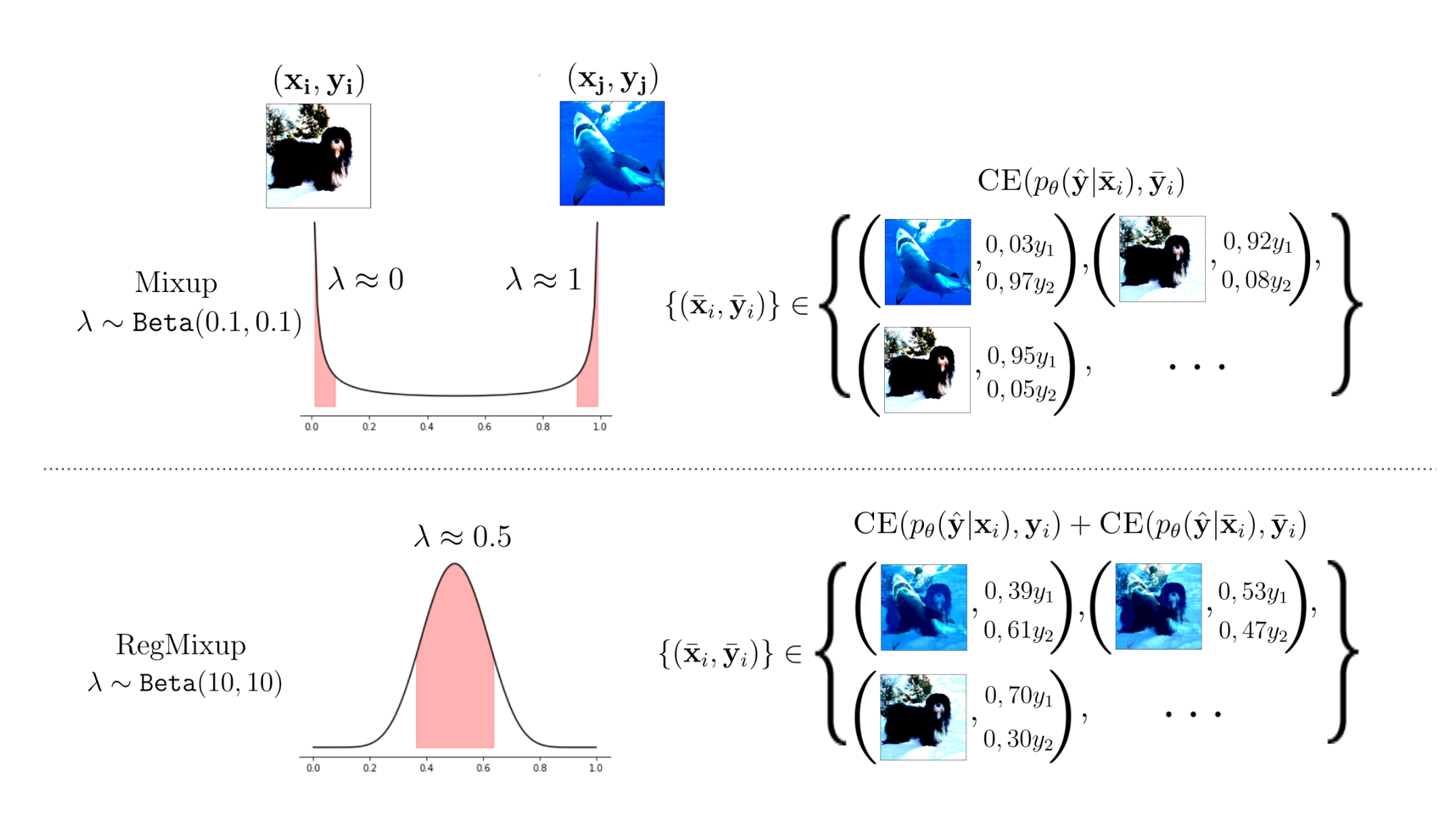
First, we take two samples $(x_i, y_i)$ and $(x_j, y_j)$ from the training set. Then, we generate a new sample $(\tilde{x}, \tilde{y})$ by taking a convex combination of the two samples with a mixup coefficient $\lambda \sim \text{Beta}(\alpha, \alpha)$ :
$$ \tilde{x} = \lambda x_i + (1 - \lambda) x_j \hspace{1cm} \tilde{y} = \lambda y_i + (1 - \lambda) y_j $$
We can then define the vicinal distribution of the mixed sample $(\tilde{x}, \tilde{y})$ as :
$$ P_{x_i, y_i} = \mathbb{E}_\lambda[( \delta {\tilde{x}_i}(x), \delta{\tilde{y}_i}(y))] \tag{3} $$
Mixup is an interesting method to consider but it possesses some limitations :
- Small $\alpha$ issues : With our setup, $\alpha \approx 1$ encourages $\tilde{x}$ to be perceptually different from $x$. Consequently, training and testing distribution will also grow appart from each other. When $\alpha \ll 1$, the mixup convex interpolation factor λ leads to a sharp peaks of 0 and 1. Therefore, Mixup will produce samples close to the initial ones (in case λ close to 1) or in the direction of another sample (in case of λ close to 0). Look at the figure below, one of the two interpolating images dominates the interpolated one. What is noticed after cross-validation of alpha is that the best values are $\alpha \approx 0.2$ which is very small. Consequently, the final sample effectively presents only a small perturbation in comparison to the original one while the vicinal distribution exploration space is much larger. We could say that Mixup does not allow to use the full potential of the vicinal distributions of the data.
- Model underconfidence : When a neural network is trained with Mixup, it is only exposed to interpolated samples. Consequently, the model learns to predict smoothed labels which is the very root cause of its underconfidence. This results in a high predictive entropy for both ID and OOD samples.
Mixup vs RegMixup, underconfidence and space exploration.
2. RegMixup in theory
Now that we have understood the path that led to RegMixup, we will explore its theoretical background and see how and why it is a good regularizer for robust AI.
While Mixup utilizes data points’ vicinal distribution only, RegMixup uses both the vicinal and the empirical one (refering respectively to VRM and ERM). This can seem far-fetched or even counter-intuitive but produces very interesting properties.
$$ P(x, y) = \frac{1}{n} \sum_{i=1}^n \left( \gamma \delta_{x_i}(x) \delta_{y_i}(y) + (1-\gamma) P_{x_i, y_i}(x, y) \right) \tag{4} $$
Here, $\gamma$ is the hyperparameter controlling the mixup between the empirical and vicinal distribution. In fact, we see that the distribution $P(x, y)$ for RegMixup is a convex combination of the empirical distribution (left term of the addition in equation 4) and the vicinal distribution defined with equations (2) and (3).
From there, we can define a new loss function $\mathcal{L}$ based on the Cross Entropy Loss ($\text{CE}$)
$$ \mathcal{L}(\hat{y}, y) = \text{CE}(p_\theta(\hat{y} \vert x), y) + \eta \text{CE}(p_\theta(\hat{y} \vert \tilde{x}), \tilde{y}) \tag{5} $$
With $ \eta \in R_{+}^{\ast} $ being the hyperparameter controlling the importance of the vicinal cross entropy sub-loss and $p_\theta$ the activation function of the model parameterized by $\theta$. In the paper, the value of $\eta$ is set to 1 and its variation seem negligible. Consequently, we will not focus on it in this blog post.
Such a model (equation 4) exhibits properties that lacked in Mixup :
- Values of $\alpha$ and underconfidence : As we explicitly add the empirical distribution to the vicinal one, the ERM term will encourage the model to predict the true labels of the training set while the VRM term, motivated by the interpolation factor $\lambda$, will explore the vicinal distribution space in a much more thorough way than what was possible with Mixup. For instance, if λ $\approx$ 0.5, a wide variety of images containing features from both the images in the pair are obtained (look at the figure). Consequently, the ERM term allows to better predict in-distribution samples while the VRM term, with a larger $\alpha$, will allow to better predict OOD samples. This is a very interesting property as it allows to have a model that is both confident and accurate.
- Prediction entropy : Through their experiments and observations, researchers found that a cross-validated value of $\alpha$ leads to a maximum likelihood estimation having high entropy for ODD samples only. While Mixup demonstrated high entropy for both ID and OOD samples, RegMixup is able to differentiate between the two. This is an highly desirable properties indicating us that RegMixup acts as a regularizer in essense.
As a preliminary conclusion, RegMixup is a very powerful, cost-efficient and simple-to-implement regularizer that allows to improve the robustness and accuracy of deep neural networks for both in-distribution and out-of-distribution samples. In the next section, we will see how to use RegMixup in practice trough a toy example.
3. RegMixup in practice (implementation)
Now, our objective will be to demonstrate the effectiveness of RegMixup through a very simple example. We will use the CIFAR-10-C dataset (corrupted version of CIFAR-10) and a standard ResNet-18 model. We will compare performances of 3 models :
- A baseline model trained with ERM
- A model trained with Mixup
- A model trained with RegMixup
To do so, we have two possibilities :
- Use the official implementation of RegMixup available on Francesco Pinto's GitHub.
- Use the torch-uncertainty library which provides a simple and efficient way to use RegMixup. Note, the library is developed by researchers from ENSTA Paris and is available on GitHub.
In this blog post, we will use the torch-uncertainty library as it is very simple to use and provides a very well-implemented version of RegMixup.
3.1. Installation
First, we need to install the torch-uncertainty library. To do so, we can use pip :
pip install torch-uncertainty
Note: If you use a gpu, torch-uncertainty will automatically install a cpu version of torch and torchvision, you can compile the following lines to install the gpu version of torch and torchvision (took from PyTorch website) :
pip unistall torch torchvision
pip3 install torch torchvision --index-url https://download.pytorch.org/whl/cu118
To check if the installation was successful, you can run the following code, it should return True if you have a gpu and False if you don’t have one :
import torch
print(torch.cuda.is_available())
3.2. Training the models with torch-uncertainty
Now that we have installed torch-uncertainty, we can train the models. First, we need to import the necessary libraries :
from torch_uncertainty import cli_main, init_args
from torch_uncertainty.baselines.classification import ResNet
from torch_uncertainty.optimization_procedures import optim_cifar10_resnet18
from torch_uncertainty.datamodules import CIFAR10DataModule
from torchvision.datasets import CIFAR10
from torchvision import transforms
from torch.nn import CrossEntropyLoss
import torch

import os
from pathlib import Path
from cli_test_helpers import ArgvContext
Then, we can define the 3 models we discussed earlier :
baseline = ResNet(num_classes=10,
                loss=CrossEntropyLoss,
                optimization_procedure=optim_cifar10_resnet18,
                version="std",
                in_channels=3,
                arch=18).cuda()

mixup = ResNet(num_classes=10,
                loss=CrossEntropyLoss,
                optimization_procedure=optim_cifar10_resnet18,
                version="std",
                in_channels=3,
                arch=18,
                mixup=True,
                mixup_alpha=0.2).cuda()

regmixup = ResNet(num_classes=10,
                loss=CrossEntropyLoss,
                optimization_procedure=optim_cifar10_resnet18,
                version="std",
                in_channels=3,
                arch=18,
                reg_mixup=True,
                mixup_alpha=15).cuda()
Before training the models, we need to define important arguments such as training parameters (epochs, estimators, etc.) and the datamodule. We can do so with the following code:
root = Path(os.path.abspath(""))

# We mock the arguments for the trainer
with ArgvContext(
    "file.py",
    "--max_epochs",
    "20",
    "--enable_progress_bar",
    "False",
    "--num_estimators",
    "8"
):
    args = init_args(network=ResNet, datamodule=CIFAR10DataModule)

net_name = "logs/reset18-cifar10"

# datamodule
args.root = str(root / "data")
dm = CIFAR10DataModule(**vars(args))
Finally, we can train the models using the cli_main function from torch-uncertainty :
results_baseline = cli_main(baseline, dm, root, net_name, args=args)
results_mixup = cli_main(mixup, dm, root, net_name, args=args)
results_regmixup = cli_main(regmixup, dm, root, net_name, args=args)
Note: If you have a gpu, you can make a slight modification to the code to use it :
- Click on
cli_mainand pressF12to go to the function definition. - Go to line 222 and replace the trainer definition by the following one :
# trainer
    trainer = pl.Trainer.from_argparse_args(
        args,
        accelerator="gpu",
        devices=1,
        callbacks=callbacks,
        logger=tb_logger,
        deterministic=(args.seed is not None),
        inference_mode=not (args.opt_temp_scaling or args.val_temp_scaling),
    )
- Save the file and you are all set.
3.3. Results
So as to compare the performances of the 3 models, we use two corrupted versions of Cifar-10-C. The first version has a corruption severity factor of 5 (slight data corruption) and the second one has a corruption severity factor of 15 (more severe data corruption). Our study contains 5 metrics : entropy, accuracy, brier score, expected calibration error (ECE) and negative log-likelihood (NLL). In our explanation, we will focus on the accuracy and entropy to keep it simple.
With corruption severity factor of 5, we obtain the following results :
| entropy | accuracy | brier | ece | nll | |
|---|---|---|---|---|---|
| baseline | 0.656294 | 0.7480 | 0.349862 | 0.032466 | 0.729336 |
| mixup | 0.640811 | 0.7578 | 0.335403 | 0.024429 | 0.703844 |
| regmixup | 0.676174 | 0.7564 | 0.340233 | 0.023135 | 0.711405 |
First of all, we can see that the accuracy is quite similar for the 3 models. This makes sense as the corruption severity factor is quite low, thus cifar-10-c is not very different from the original cifar-10. However, we can see that the entropy of the RegMixup model is higher than the one of the Mixup model. This is symptomatic of Mixup’s underconfidence. As stated previously, given the low corruption severity factor of cifar-10-c, the underconfidence of Mixup does not impact its performances in a visible manner.
With corruption severity factor of 15, we obtain the following results :
| entropy | accuracy | brier | ece | nll | |
|---|---|---|---|---|---|
| baseline | 0.615607 | 0.7402 | 0.358522 | 0.048414 | 0.750933 |
| mixup | 0.698558 | 0.7558 | 0.338540 | 0.014760 | 0.709190 |
| regmixup | 0.702599 | 0.7614 | 0.327945 | 0.008439 | 0.687550 |
Here the results are much more unequivocal. As the severity factor increases, the baseline model drops in accuracy and entropy, Mixup also drops in accuracy but increases in entropy and RegMixup increases in accuracy and entropy. Here, RegMixup has the higher entropy as the model has higher entropy for OOD samples which are more frequent at this corruption level. Mixup shows a greater delta increase in entropy due to its higher predictive entropy tendency whether or not samples are OOD or ID. Consequently, RegMixup is more confident and accurate than the Mixup model eventhough Mixup is not fully underperforming.
4. Conclusion
As a conclusion, we have seen that RegMixup is a powerful method to regularize deep neural networks. Despite being very simple and cost-effective, it is important to specify that the paper does not provide a theoretical explanation of the method. These experimental grounds are very promising but it appears important to stay cautious while utilizing RegMixup.