Robust Classifiers Energy Based Models

Unlocking the Secrets of Robust AI: How Energy-Based Models Are Revolutionizing Adversarial Training

Authors: Lucas ALJANCIC, Solal DANAN, Maxime APPERT

Introduction: The Hidden World of Adversarial Attacks

Imagine you’ve built a state-of-the-art AI model that can classify images with near-perfect accuracy. But then, someone adds a tiny, almost invisible perturbation to an image, and suddenly your model confidently misclassifies it. This is the world of adversarial attacks, where small, carefully crafted changes can fool some advanced AI systems.

In this post, we’ll dive into a groundbreaking research paper that rethinks how we train AI models to resist these attacks. By leveraging Energy-Based Models (EBMs), the authors propose a novel approach called Weighted Energy Adversarial Training (WEAT) that not only makes models more robust but also unlocks surprising generative capabilities. Let’s break it down step by step, from the basics to the big picture.

Understanding Adversarial Attacks and Robust AI

What Are Adversarial Attacks?

Adversarial attacks can be thought of as carefully crafted optical illusions for AI. By making tiny changes to an input, attackers can manipulate the model’s output, causing incorrect predictions. These perturbations are often imperceptible to the human eye but can significantly impact AI decision-making.

Technical Explanation:

Mathematically, an adversarial example $x’$ is generated by adding a small perturbation $\delta$ to an original input $x$, such that: $$x’ = x + \delta,$$ where $\delta$ is chosen to maximize the model’s prediction error, often by solving: $$\arg\max_{\delta} ; L\bigl(f(x+\delta), y\bigr) \quad \text{subject to} \quad |\delta| \le \epsilon,$$ ensuring that the perturbation remains small. Here, $f(x)$ represents the model’s prediction, $y$ is the true label, and $L$ is the loss function.

Schematic Explanation:

A simple visualization consists of two decision boundaries: one for clean samples and another distorted by adversarial perturbations. The adversarial example, though close to the clean sample in the input space, crosses the decision boundary, leading to a misclassification. This is illustrated in the following image, which showcases the adversarial perturbation technique. For example, a small amount of noise—imperceptible to humans—can be added to an image of a panda, changing its classification to a different label (e.g., from "panda" to "gibbon") with high confidence, even though the image still looks exactly like a panda to the human eye. This occurs because the noise is specifically designed to fool the model by maximizing the prediction error.

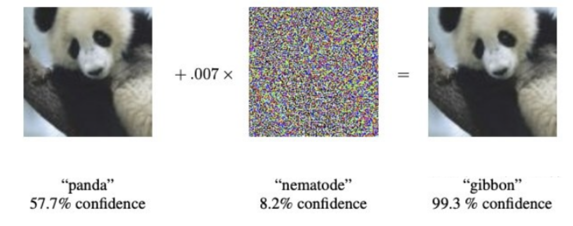
Figure 1: A small perturbation (middle) is added to a correctly classified image (left), causing a deep neural network to misclassify it with high confidence (right).

These adversarial attacks can also be used maliciously in what is known as a backdoor attack, where mislabeling during training leads to misclassification at test time. For instance, a stop sign with a slight alteration may be classified as a speed limit sign due to adversarial manipulation of the training data.

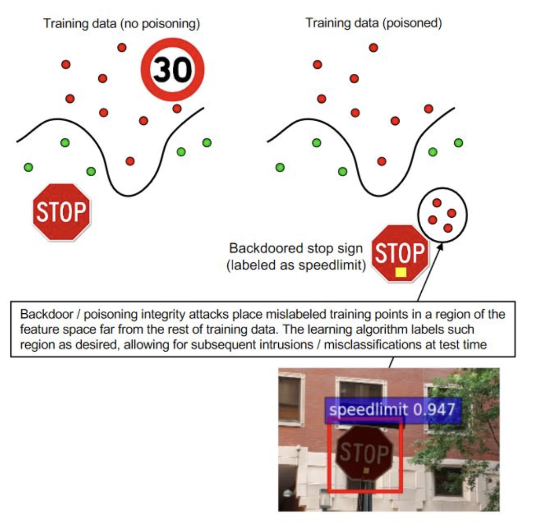
Figure 2: Poisoning the training data by mislabeling specific inputs (top right) forces the model to associate a manipulated stop sign with a speed limit sign (bottom), leading to targeted misclassification at test time.

We can easily imagine scenarios in which an adversarial attack can be critical. For example, a self-driving car misinterpreting a slightly modified stop sign as a yield sign due to adversarial perturbations could lead to catastrophic consequences.

To counteract these risks, engineers strive to build robust models where adversarial attacks are ineffective. Techniques such as feature squeezing or input transformations can sometimes remove adversarial perturbations, reducing their effectiveness.

The Quest for Robust AI: Adversarial Training

To combat adversarial attacks, researchers have developed Adversarial Training. The idea is simple: train the model on both normal data and adversarial examples (data modified to fool the model). This way, the model learns to recognize and resist these attacks.

During training, adversarial examples are generated using algorithms like Projected Gradient Descent (PGD) or the Fast Gradient Sign Method (FGSM). The model is then trained to correctly classify both clean and adversarial examples, thereby improving its resilience.

Mathematically, adversarial training involves solving the following optimization problem: $$\underbrace{\min_{\theta} E_{(x,y) \sim \mathcal{D}} \left[ \overbrace{\max_{\delta: |\delta| \le \epsilon} L\bigl(f(x+\delta;\theta), y\bigr)}^{\text{Adversarial Attack}} \right]}_{\text{Adversarial Training}}.$$ Here, the inner maximization aims to generate the worst-case perturbation $\delta$, while the outer minimization updates the model parameters $\theta$ to minimize the loss on these adversarial examples. This iterative process enhances the model’s robustness against adversarial attacks.

A schematic representation helps visualize this concept. The image below shows how a labeled or unlabeled image is used to generate an adversarial example, which is then processed by a model. The predictions of both the original and adversarial images are compared using KL divergence, with a weighted sum incorporating cross-entropy loss (for labeled images) to compute the final loss.

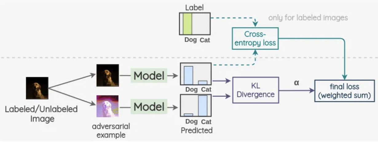
Figure 3: Representation of Adversarial Training, a model processes both clean and adversarial examples, minimizing cross-entropy loss for labeled images and KL divergence between predictions.

A useful analogy is training a security system against burglary attempts. Imagine a house protected against intruders. A basic security system might work well against naive burglars but fail against sophisticated thieves who exploit specific vulnerabilities. To strengthen the system, the homeowner continuously updates it by testing against simulated break-in attempts—much like adversarial training tests the model against simulated attacks. However, if the security system memorizes these specific attack patterns, it may remain vulnerable to novel intrusion techniques. This weakness highlights what is known as robust overfitting: the model learns to defend against the training attacks but generalizes poorly to new, unseen attacks.

To truly address robust overfitting, we must understand why it occurs. One way to do this is to analyze adversarial training through an energy-based perspective. In the next section, we explore how energy-based models offer critical insights that can help address this problem.

Energy-Based Models (EBMs) -- A New Perspective

Inspired by previous works linking adversarial training (AT) and energy-based models—which reveal a shared contrastive approach—the authors reinterpret robust discriminative classifiers as EBMs. This new perspective provides fresh insights into the dynamics of AT.

What Are Energy-Based Models?

In traditional classification, a neural network is trained to output the most likely label for an input. However, when recast as an EBM, the classifier assigns an energy to each input-label pair, $E_\theta(x,y)$, which reflects how “plausible” that combination is. In this framework, lower energy indicates that the model is more confident the input belongs to that class. EBMs rely on the assumption that any probability density function $p(x)$ can be represented via a Boltzmann distribution: $$p_\theta(x) = \frac{\exp\bigl(-E_\theta(x)\bigr)}{Z(\theta)}$$,

where $E_\theta(x)$ is the energy function mapping each input $x$ to a scalar value, and $Z(\theta) = \int \exp\bigl(-E_\theta(x)\bigr) , dx,$ is the normalizing constant ensuring that $p_\theta(x)$ is a valid probability distribution.

Similarly, the joint probability of an input and a label can be defined as: $$p_\theta(x,y) = \frac{\exp\bigl(-E_\theta(x,y)\bigr)}{Z’(\theta)}$$,

which leads to the formulation of a discriminative classifier: $$p_\theta(y \mid x) = \frac{\exp\bigl(-E_\theta(x,y)\bigr)}{\sum_{k=1}^{K} \exp\bigl(-E_\theta(x,k)\bigr)}.$$

In this context, energy serves as a measure of confidence for both the input-label pair and, when marginalized over labels, the input itself:

Adversarial Attacks Through the Energy Lens

An intriguing insight from the paper is that adversarial attacks can be interpreted by examining how they alter the energy landscape. Recall that the cross-entropy loss can be written in terms of energy as: $$L_{CE}(x,y;\theta) = -\log p_\theta(y\mid x) ;=; E_\theta(x,y) - E_\theta(x),$$ implying that an attack impact the loss—by modifying both $E_\theta(x,y)$ and $E_\theta(x)$.

Untargeted Attacks.

These attacks aim to make the classifier output any incorrect label. They raise the joint energy $E_\theta(x,y)$ (making the model to "dislike" the correct label) while lowering the marginal energy $E_\theta(x)$. Consequently, the adversarial example looks very “natural” (low $E_\theta(x)$) yet becomes unrecognizable for the true label (high energy).

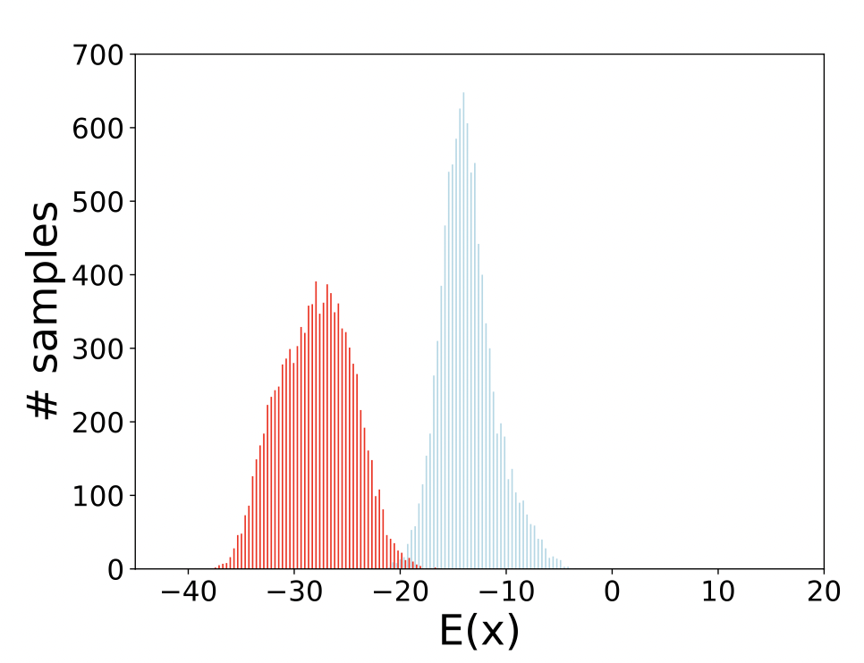
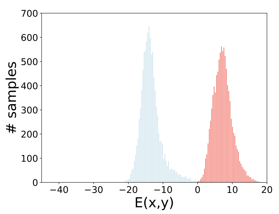
Figure 4: PGD Untargeted attacks: (Above) Distributions of $(E_\theta(x))$; (Below) Distributions of $(E_\theta(x, y))$. Blue indicates natural data, red indicates adversarial data.

Targeted Attacks.

These attacks force the classifier to predict a specific (incorrect) label $t$. The adversary perturbs $x$ to minimize the energy for the target label $E_\theta(x,t)$, thereby steering the classifier’s decision toward $t$ but raise $E_\theta(x)$ overall, making the input look out-of-distribution despite being confidently misclassified as $t$.

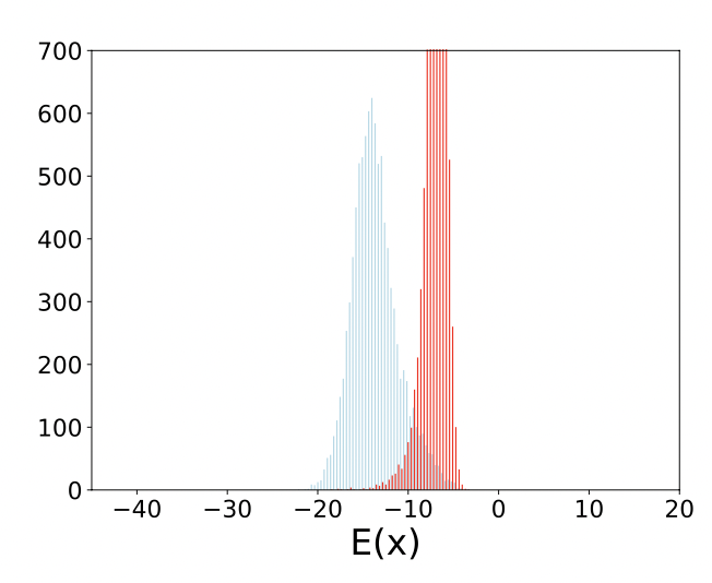
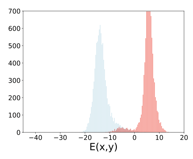
Figure 5: APGD Targeted attacks: (Above) Distributions of $(E_\theta(x))$; (Below) Distributions of $(E_\theta(x, y))$. Blue indicates natural data, red indicates adversarial data.

By revealing how each attack reshapes the energies of clean vs. adversarial examples, the authors highlight distinct patterns for untargeted and targeted strategies—informing more effective defenses.

Energy-Based Insights on Robust Overfitting

Overfitting means a model excels on training data but falters on unseen examples. In the robust setting, this manifests when a network memorizes the specific adversarial perturbations seen during training, yet struggles with new adversarial attacks. The authors reveal that robust overfitting is closely linked to a widening energy gap between clean and adversarial samples. As adversarial training progresses, the energy $E_\theta(x)$ of natural (clean) examples and the energy $E_\theta(x^\ast)$ associated with their adversarially perturbed versions diverge significantly. Surprisingly, even if a sample is “easy” (i.e., it has a low loss and the model is highly confident), only minimal perturbations are needed to flip its label due to the model’s over-confidence. These weaker perturbations, paradoxically, cause a larger distortion in the energy landscape, so that a slight adversarial change on a low-loss sample can result in a substantial discrepancy between the natural and adversarial energies.

TRADES: Aligning Clean and Adversarial Energies

TRADES (TRadeoff-inspired Adversarial DEfense via Surrogate-loss minimization) is a refined adversarial training approach that adds a term to the standard loss, ensuring that a model’s predictions on a clean input $x$ remain close to those on its adversarially perturbed version $x+\delta$. When expressed in energy terms, this extra term aligns the energies of natural and adversarial samples, thereby reducing robust overfitting. In essence, TRADES enforces similar energy values for $x$ and $x+\delta$, creating a smoother energy landscape and helping the model generalize more effectively against unseen attacks.

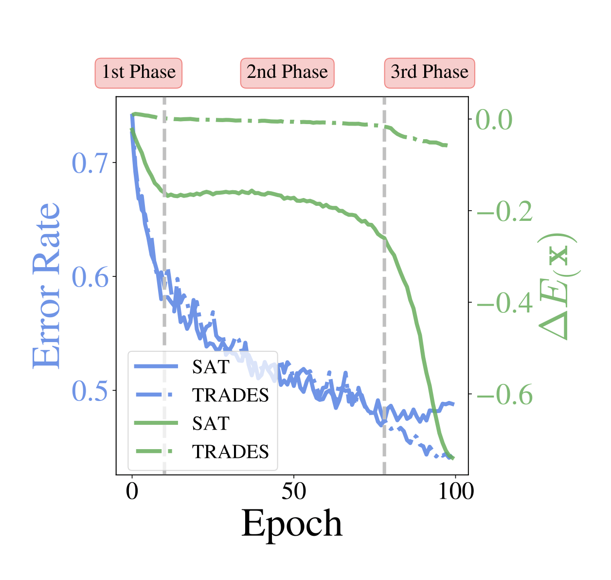
Figure 6: While SAT (line curve) experiences a steep divergence between clean and adversarial energies ($\Delta E_\theta(x)$ = $E_\theta(x)$ - $E_\theta(x^\ast)$ ) in the 3rd phase (leading to robust overfitting), TRADES (dashed curve) maintains a relatively constant energy gap. This smoother alignment mitigates overfitting and improves robustness.

One of the key empirical observations is that top-performing robust classifiers tend to exhibit a smooth energy landscape around natural data points. Concretely, the energies $E_\theta(x)$ and $E_\theta(x+\delta)$ remain closer in these models and this alignment strongly correlates with improved adversarial defense.

To sum up, these insights clarify that robust overfitting is not merely about memorizing specific adversarial examples, but rather about how the model’s internal energy representation becomes distorted. When the gap between $E_\theta(x)$ and $E_\theta(x+\delta)$ grows, the model’s ability to generalize its robustness to new attacks is compromised. These observations deepen our understanding of adversarial dynamics and informed the strategy for effective robust training methods WEAT, as described in the following section.

Weighted Energy Adversarial Training (WEAT)

Main Principle of WEAT

The authors propose WEAT, a novel method that weights training samples based on their energy. WEAT relies on Energy-Based Models (EBMs) to measure the model’s "confidence":

• Marginal Energy $E_\theta(x) = -\log \sum_k \exp(\theta(x)[k])$: The lower it is, the more "probable" the input $x$ is according to the model.

• Joint Energy $E_\theta(x, y) = -\log \exp(\theta(x)[y])$: Measures the confidence for a specific class $y$.

The article classifies samples according to their energy into three categories:

1. High-energy samples ($E_\theta (x) > -3.87$): These are difficult examples, close to decision boundaries. WEAT gives them more weight because they help the model learn better.

2. Low-energy samples ($E_\theta (x) \leq -11.47$): These are easy examples. WEAT gives them less weight to prevent overfitting.

3. Intermediate samples (between these two thresholds)

Key Idea: Samples with high energy (hard to classify) are crucial for robustness, while those with low energy (easy) risk causing overfitting. Therefore, WEAT weights them differently:

$$\text{weight}(x) = \frac{1}{\log(1 + \exp(|E_\theta(x)|))}$$

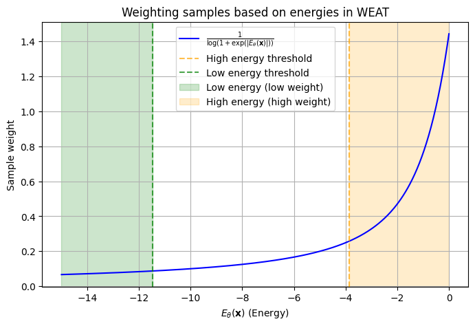
Figure 7: Weighting Visualization.

WEAT in details

The core formula of WEAT is an improvement of TRADES by introducing a dynamic weighting weight$(x)$ based on the energy $E_\theta(x)$. WEAT combines:

• Cross-entropy loss (CE): Standard classification performance measure. It contains $E_{\boldsymbol{\theta}}(\mathbf{x}, y) - E_{\boldsymbol{\theta}}(\mathbf{x})$. When this term is minimized, it allows to "dig" the valleys representing the good predictions (low energy = high confidence). For the correct class y, $E_{\boldsymbol{\theta}}(\mathbf{x}, y)$ becomes "lower" than $E_{\boldsymbol{\theta}}(\mathbf{x})$.

• KL divergence: Controls the gap between predictions on natural data $p(y|x)$ and adversarial data $p(y|x^\ast)$ with the marginal term $E_{\boldsymbol{\theta}}(\mathbf{x}) - E_{\boldsymbol{\theta}}(\mathbf{x}^\ast)$. By minimizing this gap, the model smooths the energy landscape and flattens out disturbed areas.

WEAT formula:

$$L_{\text{WEAT}} = \underset{\text{Weighting}}{\boxed{\text{weight}(x)}} \cdot \left[ \underset{\text{Standard Loss}}{\boxed{L_{\text{CE}}(x, y)}} + \beta \cdot \underset{\text{Robust Regularization}}{\boxed{\text{KL}(p(y|x) || p(y|x^\ast))}} \right] $$

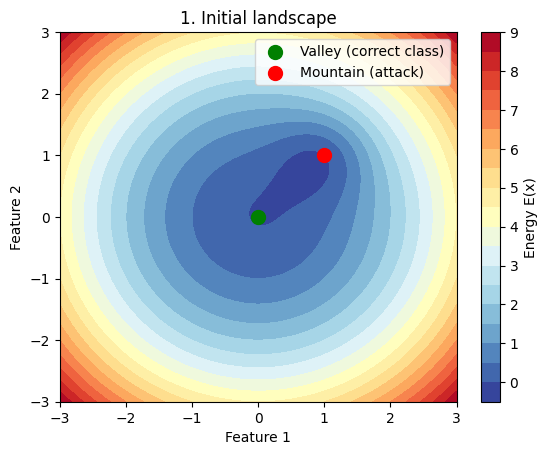
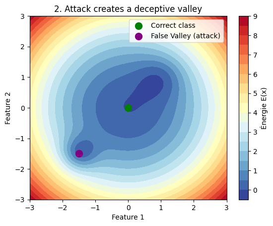
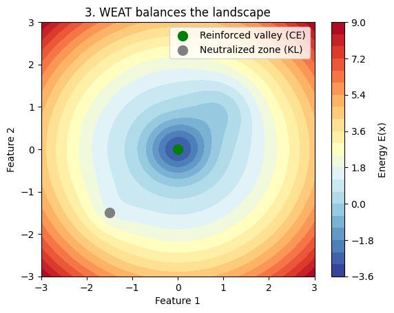
Figure 8: Diagram of WEAT dynamics

The figure above highlights the trade-off with the $\beta$ coefficient for regularization to maintain a smooth energy landscape despite adversarial attacks.

While not the main focus of this article (to avoid technical overload), WEAT also demonstrates remarkable performance in image generation through its integration with Stochastic Gradient Langevin Dynamics (SGLD). On standard benchmarks like CIFAR-10, WEAT matches the performance of hybrid models such as JEM while offering superior robustness (see Table 2c in the paper).

Conclusion: A New Era for Robust AI

Why This Matters

This research isn’t just about making AI models more robust. It’s about fundamentally understanding how these models work and how we can improve them. By rethinking adversarial training through the lens of EBMs, the authors have opened up new possibilities for both robustness and generative modeling. As AI continues to evolve, approaches like WEAT will be crucial for building models that are both accurate and secure. Surely, this type of model will play a key role in improving trust in critical technologies such as autonomous vehicles.

Potential Societal Impact

Although robust models are often considered safe from adversarial attacks, their susceptibility to inversion poses a privacy risk. Because robust classifiers can be interpreted as energy-based models, they capture substantial information about their training data—including its distribution and structure. This makes it possible, using inversion techniques, to reconstruct or approximate the original training data. If sensitive information (e.g., personal data, proprietary content, or other confidential details) is exposed, it could lead to significant privacy breaches with broader societal implications.

References

Sik-Ho Tsang. Review: Virtual Adversarial Training (VAT). Apr 21, 2022. Available at: https://sh-tsang.medium.com/review-virtual-adversarial-training-vat-4b3d8b7b2e92.

Gaudenz Boesch. Attack Methods: What Is Adversarial Machine Learning?. December 2, 2023. Available at: https://viso.ai/deep-learning/adversarial-machine-learning/.

Mujtaba Hussain Mirza1, Maria Rosaria Briglia, Senad Beadini, and Iacopo Masi. Shedding More Light on Robust Classifiers under the lens of Energy-based Models. 2025. Available at: https://arxiv.org/abs/2407.06315.