Packed Ensembles

Packed-Ensembles

The base network and Packed-Ensembles

Packed-Ensembles (PE) is a technique for designing and training lightweight ensembles of neural networks. It is based on the idea of using grouped convolutions to create multiple subnetworks within a single network. These subnetworks are trained independently, which helps to improve the efficiency of the ensemble.

Benefits of Packed-Ensembles

Packed-Ensembles offer several benefits over traditional ensemble methods, including:

• Efficiency: Packed-Ensembles are more efficient than traditional ensembles in terms of memory usage and training time. This is because they use grouped convolutions to share parameters between the subnetworks.

• Accuracy: Packed-Ensembles can achieve accuracy levels that are comparable to traditional ensembles.

• Calibration: Packed-Ensembles are well-calibrated, meaning that their predicted probabilities are accurate reflections of the true probabilities.

• Out-of-distribution (OOD) detection: Packed-Ensembles are good at detecting out-of-distribution data, which is data that comes from a different distribution than the data that the model was trained on.

Comparison to other ensemble methods

The paper compares Packed-Ensembles to several other ensemble methods, including Deep Ensembles, BatchEnsemble, MIMO, and Masksembles. The paper found that Packed-Ensembles are more efficient than all of these methods, and they achieve comparable accuracy on most tasks.

Packed-Ensembles (PE) is a method for designing and training lightweight ensembles of neural networks. It aims to improve efficiency while maintaining accuracy and other desirable properties. This technique achieves this by leveraging grouped convolutions to create multiple subnetworks within a single network, enabling them to be trained independently.

Understanding Convolutional Layers and Grouped Convolutions:

• Convolutional Layers: These are the backbone of Convolutional Neural Networks (CNNs), performing filtering operations on input data using learnable filters (kernels). Mathematically, the output of a convolutional layer, denoted by $z_{j+1}$, is calculated as follows:

$z^{(j+1)}(c,:,:) = (h^j \otimes \omega^j)(c,:,:) = \sum_{k=0}^{C_{j}-1} \omega^j(c, k,:,:) \star h^j(k,:,:)$

where:

• $c$ represents the channel index

• $h^j$ denotes the input feature map

• $ω^j$ represents the weight tensor (kernel)

• $⋆$ denotes the 2D cross-correlation operator

• Grouped Convolutions: This technique allows training multiple subnetworks within a single network by dividing the channels of feature maps and weight tensors into groups. Each group is processed by a separate set of filters, essentially creating independent subnetworks. The mathematical formulation for grouped convolutions is given by:

$$ z^{(j+1)}(c,:,:) = \left( h^j \otimes \omega^j_{\gamma} \right) (c,:,:) = \sum_{k=0}^{\frac{C_{j}}{\gamma}-1} \omega^j_{\gamma} (c, k,:,:) \star h^j \left( k + \left\lfloor \frac{c}{C_{j+1}/\gamma} \right\rfloor \frac{C_{j}}{\gamma}, :,:\right) $$

where:

• $γ$ represents the number of groups
• $C_{j+1}$ and $C_j$ denote the number of output and input channels, respectively.

The formula states that a grouped convolution layer is mathematically equivalent to a standard convolution where the weights are selectively applied using a binary mask $\text{mask}_{m}^j$ $\in \{{ 0, 1 \}}^{C_{j+1} \times C_j \times s_j^2}$ with $s_j^2$ the kernel size squared of the layer $j$. Each element in $\text{mask}_{m}^j$ is either 0 or 1.

The condition $\text{mask}_{m}^j(k, l, :, :) = 1$ happens only if $\left\lfloor \frac{l}{C_{j}/\gamma} \right\rfloor = \left\lfloor \frac{k}{C_{j+1}/\gamma} \right\rfloor$ for each group $m \in [|0, \gamma - 1 |]$

• Complete Mask and Convolution:
  • $\text{mask}^j = \sum_{m=0}^{{\gamma}-1}\text{mask}_{m}^j$ : This combines the masks for all groups ($m$) into a single $\text{mask}^j$ for layer $j$.
  • $z^{j+1} = h^j \otimes (ω^j ◦ \text{mask}^j)$: This rewrites the grouped convolution operation. Here:
    • $z^{j+1}$: Output feature map of the layer.
    • $h^j$: Input feature map.
    • $ω^j$: Convolution weights for layer j.
    • $\otimes$: Denotes convolution operation.
    • $◦$: Denotes Hadamard product (element-wise multiplication).

In simpler terms:

• Grouped convolution divides the input channels and weights into groups.
• A separate mask is created for each group, ensuring elements within a group are aligned.
• These masks effectively turn specific weights to zero during the convolution, essentially selecting which weights contribute to the output for each group.
• The final convolution is equivalent to applying the original weights element-wise multiplied by the combined mask.

This section delves into Deep Ensembles (DE), a technique for image classification tasks.

Deep Ensembles

Setting the Scene

We have a dataset $D$ containing pairs of images and their corresponding labels:

• $x_i$: Represents an image sample with dimensions $C0 \times H0 \times W0$ (likely referring to color channels, height, and width).
• $y_i$ : One-hot encoded label representing the class of the image ($NC$ total classes).

The dataset is assumed to be drawn from a joint distribution $P(X, Y)$.

A neural network $f_\theta$ processes the images and predicts their class labels. This network has learnable parameters denoted by $\theta$.

• $\hat{y}_i = f_θ(xi)$: The predicted class label for image $x_i$ based on the network with parameters $θ$.

Traditional Approach:

The model predicts probabilities for each class using a Multinoulli distribution. These probabilities are treated as point estimates, meaning they represent the most likely class without considering uncertainty.

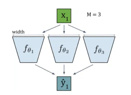
Introducing Deep Ensembles

DE works by training multiple Deep Neural Networks (DNNs) $M$ with random initializations. These DNNs are denoted by $θ_m$ for the $m-th$ network ($0$ to $M-1$).

The ensemble prediction is obtained by averaging the predictions of all $M$ DNNs as shown in the equation below:

$$ P(y_i|x_i, D) = M^{-1} \sum_{m=0}^{M-1} P(y_i|x_i, \theta_m) $$

This essentially combines the outputs of multiple networks to create a more robust prediction.

In simpler terms, DE trains multiple neural networks with slight variations and combines their predictions to get a more reliable estimate, including the level of uncertainty in the prediction.

Building Packed-Ensembles:

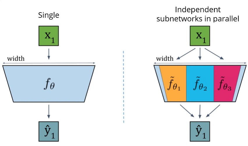
Packed-Ensembles combine the concepts of Deep Ensembles (ensembles of multiple independent DNNs) and grouped convolutions. Here’s how it works:

• Subnetworks: The ensemble is formed by creating $M$ smaller subnetworks within the main network architecture. These subnetworks share the same structure but have independent parameters due to the use of grouped convolutions.
• Hyperparameters: Packed-Ensembles are defined by three hyperparameters:
  • $α$ (alpha): expansion factor that scales the width of each subnetwork (compensates for the decrease in capacity due to using fewer parameters).
  • $M$: number of subnetworks in the ensemble (represents the ensemble size).
  • $γ$ (gamma): number of groups for grouped convolutions within each subnetwork (introduces another level of sparsity).

Mathematical Implementation:

The output of a Packed-Ensemble layer is calculated by averaging the predictions from each subnetwork, as shown in the following equation:

$$ \hat{y} = M^{-1} \sum_{m=0}^{M-1} P(y|\theta_a^m, x) \quad \text{with} \quad \theta_a^m = ({\omega_j^{\alpha} \circ \text{mask}_{m}^j})_j $$

where:

• $\hat{y}$ represents the ensemble’s predicted label
• $P(y|θ_a^m, x)$ denotes the probability of class $y$ given the input $x$ and the parameters $θ_a^m$ of the $m-th$ subnetwork
• $\theta_a^m = ({\omega_j^{\alpha} \circ \text{mask}_{m}^j})_j$ represents the parameters of the $m-th$ subnetwork, obtained by applying element-wise multiplication ($∘$) between the expanded weights ($\omega_j^{\alpha}$) and the group mask ($\text{mask}_{m}$) for each layer $j$

Implementation

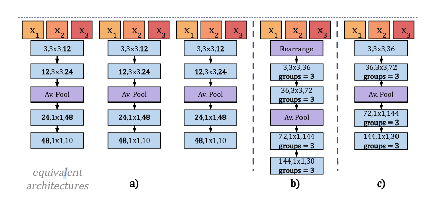
Equivalent architectures for Packed-Ensembles

The authors proposed a method for designing efficient ensemble convolutional layers using grouped convolutions. This approach exploits the parallelization capabilities of GPUs to accelerate training and inference. The sequential training architecture is replaced with parallel implementations, as shown in the part b and c of the figure above. This figure summarizes equivalent architectures for a simple ensemble of M=3 neural networks with three convolutional layers and a final dense layer. In these implementations, feature maps are stacked on the channel dimension (denoted as rearrange operation). This results in a feature map of size M × Cj × Hj × Wj, regrouped by batches of size B × M, where B is the batch size of the ensemble. To maintain the original batch size, the batch is repeated M times after rearrangement. Grouped convolutions with M groups and γ subgroups per subnetwork are employed. Each feature map is processed independently by each subnetwork, resulting in separate outputs. Grouped convolutions are used throughout to ensure gradients remain independent between subnetworks. Other operations, like Batch Normalization, can be applied if they are groupable or act independently on each channel. The figure below illustrates the masks used to encode Packed Ensembles for M=2 and M=2 with γ=2. Finally, implementations (b) and (c) of the figure above are equivalent. A standard convolution can replace the initial steps (rearrangement and first grouped convolution) if all subnetworks receive the same images simultaneously.

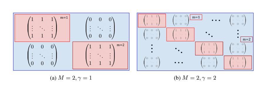
Diagram representation of a subnetwork mask: maskj, with M = 2, j an integer corresponding to a fully connected layer

The experiment section evaluates the Packed-Ensembles (PE) method on classification tasks. Here are the key points:

• Datasets: CIFAR-10, CIFAR-100, and ImageNet are used for various complexity levels.
• Architectures: PE is compared on ResNet-18, ResNet-50, Wide ResNet-28-10 against Deep Ensembles, BatchEnsemble, MIMO, and Masksembles.
• Metrics: Accuracy (%), Negative Log-Likelihood (NLL), Expected Calibration Error (ECE) for calibration, and Areas Under Precision-Recall (AUPR) and ROC (AUC) curves for Out-of-Distribution (OOD) detection are used.
• Implementation Details: Softmax probabilities from all subnetworks are averaged for prediction. Maximum value of the output vector is considered the class. SVHN dataset is used for OOD detection on CIFAR-10/100. Mutual Information (MI) is used as a criterion for ensemble techniques on ImageNet-O and Texture datasets. ImageNet-R is used to evaluate robustness under distribution shift.
• Code: PyTorch-Lightning framework is used for implementation.

The experiment results show that Packed-Ensembles (PE) achieves similar performance to Deep Ensembles (DE) on classification tasks, but with lower memory usage. Here are the key findings:

• CIFAR-10/100:
  • PE performs similarly or slightly better than DE on OOD detection and classification (especially with larger architectures like ResNet-50 and Wide ResNet).
  • Smaller architectures (ResNet-18) might not have enough capacity for PE to perform as well on CIFAR-100.
• ImageNet:
  • PE improves uncertainty quantification for OOD detection and distribution shift compared to DE and single models.
  • PE achieves better accuracy with a reasonable increase in training and inference cost.

These results suggest that PE is a memory-efficient alternative to DE for tasks requiring good uncertainty estimation.

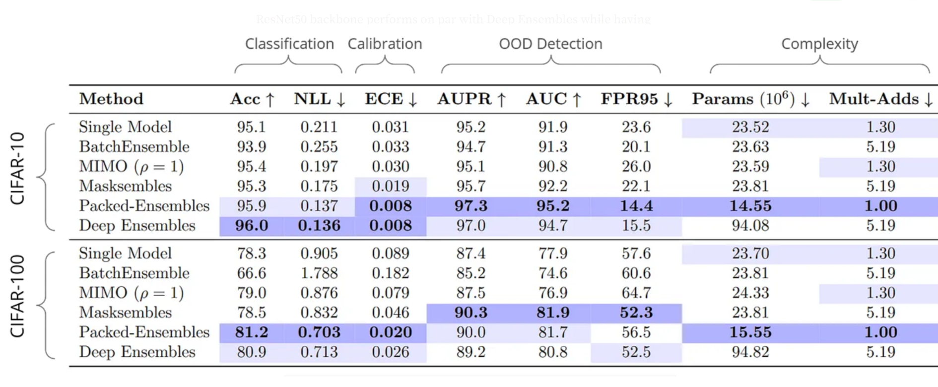
Packed-Ensembles of ResNet50 performance on CIFAR-10 and CIFAR-100

This section emphasizes the ethical considerations of the research. Here are the key points:

• Goal: This research proposes a method to improve uncertainty estimation in deep learning models.
• Limitations: The authors acknowledge limitations, particularly for safety-critical systems (systems where failure can have severe consequences). Even though the method aims to improve reliability, it’s not ready for such applications.
• Concerns: The text mentions limitations explored in the experiments. These limitations highlight the need for further validation and verification before real-world use, especially concerning robustness in various scenarios like:
  • Unknown situations
  • Corner cases (uncommon but important situations)
  • Adversarial attacks (attempts to intentionally mislead the model)
  • Potential biases in the model
• Overall: The authors advocate for responsible use of the method and emphasize the importance of further research before deploying it in safety-critical systems.

We attempted to reproduce the experiment outlined in the tutorial available at https://torch-uncertainty.github.io/auto_tutorials/tutorial_pe_cifar10.html which trains a Packed-Ensemble classifier on the CIFAR-10 dataset. The tutorial details a step-by-step approach, including:

1. Data Loading and Preprocessing: Utilizing torchvision to load the CIFAR-10 dataset and performing normalization on the images.
2. Packed-Ensemble Definition: Defining a Packed-Ensemble model with M=4 subnetworks, alpha=2, and gamma=1, built upon a standard convolutional neural network architecture.
3. Loss Function and Optimizer: Employing Classification Cross-Entropy loss and SGD with momentum for optimization during training.
4. Training: Training the Packed-Ensemble model on the CIFAR-10 training data.
5. Testing and Evaluation: Evaluating the trained Packed-Ensemble on the CIFAR-10 test data, with a focus on uncertainty quantification and OOD (Out-of-Distribution) detection performance.

Experimental Runs and Observations:

Test 1:

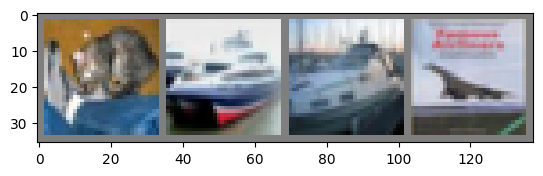
GroundTruth: cat ship ship plane

The predicted labels are: cat ship ship ship

Test 2:

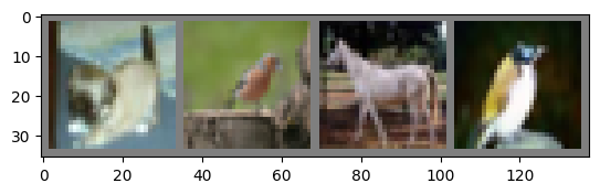
GroundTruth: dog bird horse bird

The predicted labels are: dog frog car dog

Test 3:

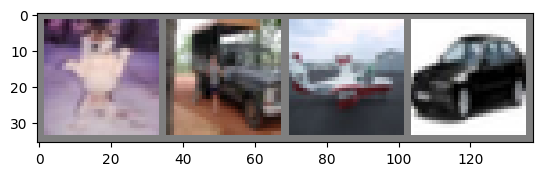
GroundTruth: dog truck plane car

The predicted labels are: dog horse ship truck

Challenges and Limitations:

A significant limitation of the tutorial is the lack of guidance on evaluating the model’s performance. Without a defined evaluation metric (e.g., accuracy, precision, recall), it’s challenging to determine the overall effectiveness of the trained Packed-Ensemble. While the provided test results show inconsistencies between ground truth labels and predictions, a quantitative evaluation metric is necessary to draw more concrete conclusions.