To update or not to update? Neurons at equilibrium in deep models
To update or not to update? Neurons at equilibrium in deep models
Author: Alexis WINTER Augustin CREUSILLET
Table of content
This is a blog post about the paper To update or not to update? Neurons at equilibrium in deep models, published by A. Bgragagnolo et al. in 2022 and available [here]https://proceedings.neurips.cc/paper_files/paper/2022/file/8b2fc235787852ead92da2268cd9e90c-Paper-Conference.pdf).
Introduction
Background
Recent advances in deep learning have undeniably propelled the field to unprecedented heights, revolutionizing various domains from computer vision to natural language processing. However, these strides forward have not come without a significant toll on computational resources. As models grow increasingly complex, the demand for computational power has surged exponentially. One of the most expensive tasks in deep learning is undoubtedly the training of models. This process entails iteratively adjusting millions or even billions of parameters to minimize a predefined loss function, requiring extensive computational power and time-intensive operations. This process poses challenges in terms of both affordability and environmental sustainability, highlighting the need for innovative solutions to make deep learning more efficient and accessible in the face of escalating computational demands.
This paper tries to focus on the overall behavior of neurons, leveraging the notion of neuronal equilibrium (NEq). When a neuron reaches a state of equilibrium, indicating that it has learned a particular input-output mapping, it ceases its updates. The result is that we can reduce the number of operations needed for the computation of the backpropagation and optimizer and thus reduce the number of resources necessary for the model.
Related works
Pruning strategies
Pruning strategies consist in the systematic removal of redundant or less important parameters, connections or units within a model to improve efficiency and reduce computational complexity. These strategies are inspired by the biological concept of pruning, where unnecessary connections in neural networks are eliminated to enhance neural efficiency. Pruning can take various forms, including magnitude-based pruning, where parameters with small weights are pruned, or structured pruning, which removes entire neurons, channels, or layers based on specific criteria. Pruning strategies effectively reduce the model size leading to a more frugal and compact model With the development of computational resources and the creation of more complex model, pruning strategies such as dropout are being exploited again.
Despite its effectiveness in reducing model size and improving inference efficiency, pruning strategies typically do not alleviate the computational complexity associated with training neural networks. While pruning removes parameters or connections during the inference phase, the training process still requires the full model to be trained initially, often resulting in high computational demands. In fact, pruning can even increase training complexity due to the need for additional iterations to fine-tune the remaining parameters and adapt the model to compensate for the pruned components. Consequently, while pruning offers significant benefits in terms of model deployment and inference efficiency, it does not directly address the computational burden of training models.
Lottery ticket hypothesis
The lottery ticket hypothesis is a concept in deep learning that suggests that within a dense neural network, there exist sparse subnetworks, or “winning tickets,” that are capable of achieving high accuracy when trained in isolation. These winning tickets are characterized by having a small subset of well-initialized weights, which when pruned to remove the remaining connections, can maintain or even surpass the performance of the original dense network.
The hypothesis was introduced by Jonathan Frankle and Michael Carbin in 2018. They conducted experiments demonstrating that randomly-initialized, dense neural networks contain subnetworks that can achieve high performance when trained properly. These subnetworks or winning tickets tend to emerge during the training process and possess a specific initialization that allows them to be effectively trained within the broader network.
The significance of the lottery ticket hypothesis lies in its potential to improve the efficiency of training deep neural networks. By identifying these winning tickets and training only the sparse subnetworks, researchers can reduce computational costs associated with training while maintaining or even improving model accuracy. This concept has led to the development of pruning techniques aimed at discovering these winning tickets and accelerating the training process.
NEq
Neuronal equilibrium
The concept of neuronal equilibrium aims to detect when a neuron reaches a state of equilibrium, indicating that it has learned a particular input-output mapping. The idea is to understand when the neuron has reach a configuration in which he does not require further updates.
To assess this we can evaluate cosine similarity between all the outputs of the $i$-th neuron at time $t$ and at time $t-1$ for the whole validation set $\Xi_{val}$ as follows:

The neuron $i$-th reaches the equilibrium when $(\phi_{i})_t$ stops evolving. In this sense to know when the neuron has reached the equilibrium we need to detect when :
$$\lim_{t\rightarrow \infty} \phi_{i}^t = k,$$
Since it is not trivial to assess this statment we prefer to work with variations of $(\phi_{i})_t$ that can be defined as :
\begin{equation} v_{\Delta \phi_i}^t = \Delta \phi_i^t - \mu_{eq} v_{\Delta \phi_i}^{t-1}, \end{equation}
With $\mu_{eq}$ the momentum coefficient.
This only lead to a reformulation of the problem as the equilibrium is reached when we have : $$\Delta \phi_i^t \rightarrow 0$$
Since we want to track the evolution of $\Delta \phi_i^t$ over time we introduce the velocity of the variations: $$ v_{\Delta \phi_i}^t = \Delta \phi_i^t - \mu_{eq} v_{\Delta \phi_i}^{t-1}, $$
With $\mu_{eq}$ the momentum coefficient.
Rewrited:

We need to have $$\mu_{eq} \in [0; 0.5]$$ to prevent the velocity from exploding.
Finally we can set the condition for the neuron to be at the equilibrium as: \begin{equation} \left| v_{\Delta \phi}^t \right | < \varepsilon,~~~~~\varepsilon \geq 0. \end{equation}
It is important to know that this relation might not hold for all $t$ since there could be an instant $t’ < t$ where the relation does not hold anymore and the neuron is attracted to a new state and need to be updated again.
Training scheme
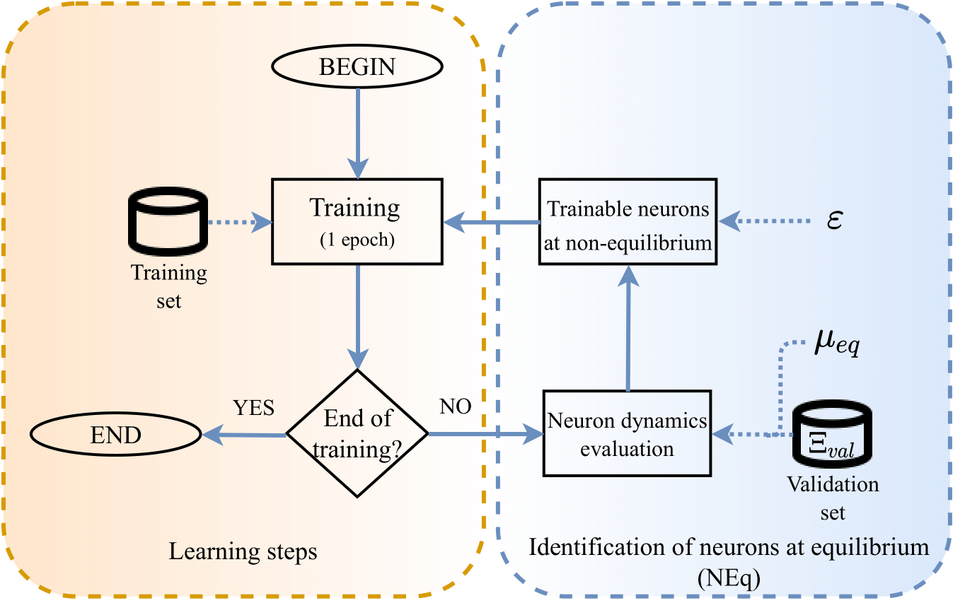
The training scheme can be presented according to this scheme:

At the first epoch each neuron is considered to be at non-equilibrium. After the first epoch the training scheme can be described as followed:
- An epoch of training is made for all trainable neurons on the training set.
- The training either stops due to the end of training criterion being met or continues to the next step.
- The velocity of the similarities is evaluated for every neuron.
- The set of trainable neurons is determined for the next step according to the equilibrium criterion.
Comparing with regular training, we can see two more hyper-parameters:
- $\epsilon$ which determines the threshold at which a neuron is considered to be at equilibrium according to the velocity of the similarities.
- $\mu_{eq}$ which intervenes into the calculation of the velocity of the similarities.
Experiments
SGD vs Adam

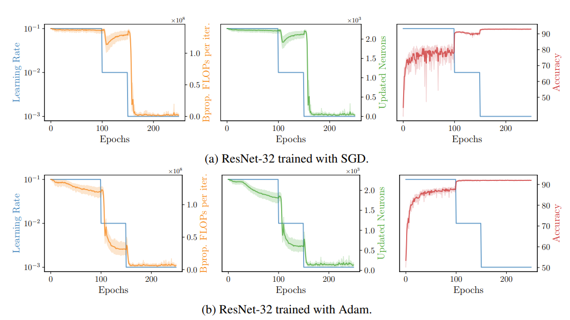
The authors conducted an experiment comparing two training methods for a ResNet-32 neural network on the CIFAR-10 dataset. The methods compared are SGD (Stochastic Gradient Descent) with momentum and Adam, which are both optimization algorithms used to update network weights iteratively.
In the experiment, the authors observe the FLOPs required for a back-propagation step and the number of updated neurons during training. They note that at high learning rates, more neurons are trained and more FLOPs are required. This is attributed to the network not being at equilibrium—essentially, the network parameters are still very fluid and subject to change, thus requiring more computation.
As training progresses and the learning rate is reduced, fewer neurons need updating, as the network moves towards its final, more stable configuration. The authors find that Adam brings the network towards this equilibrium faster than SGD, but also note that in this specific task, SGD achieves a slightly higher final accuracy than Adam. This may suggest that while Adam is efficient in reaching a state where few neuron weights are updated, SGD’s ability to explore the solution space more thoroughly leads to a better generalization on the test data.
The experiment also highlights an interesting behavior at the first learning rate decay around epoch 100 for SGD. The number of updated neurons decreases and then increases, which is not observed with Adam. This difference illustrates the contrasting approaches of the two optimizers: SGD, by reducing the learning rate, encourages continued exploration, which temporarily stabilizes the network until it adjusts to the new learning rate and begins exploring again. Adam, with its adaptive learning rate for each parameter, does not exhibit this behavior because it consistently steers the network towards a stable state.
Distribution of $\phi$ & choice of $µ_{eq}$

The paper also discusses the distribution of $\phi$ and the choice of a parameter called $µ_{eq}$ during the training of neural networks.
The parameter $\phi$ measures the cosine similarity between the outputs of a particular neuron at two consecutive training epochs, over the validation set. It is used to determine if a neuron’s output has reached equilibrium, meaning its outputs do not significantly change over successive epochs. If $\phi$ equals 1, it indicates that the neuron’s output is stable across the epochs, signifying it has reached equilibrium.
The paper further discusses the dynamics of neurons as they approach equilibrium. To quantify this, they introduce a metric called ∆φ, which is the difference in the $\phi$ values across epochs, and $v_{∆\phi}$, which measures the velocity of this change considering a momentum coefficient $µ_{eq}$. This coefficient is important as it determines how much previous changes impact the current measurement of the equilibrium state.
By examining different values for $µ_{eq}$, the paper finds that setting $µ_{eq}$ to 0.5 provides a good compromise, as it ensures a balance between memory of past variations and responsiveness to new changes. This finding is illustrated in the paper’s Figure 5, which shows the distribution of $\phi$, $∆\phi$, and $v_{∆\phi}$ for a ResNet-32 model trained on CIFAR-10.
In summary, the authors find that a neuron is at equilibrium if the velocity of the similarity changes, considering the momentum, is below a certain threshold. They also observe that during training, even after reaching equilibrium, neurons may occasionally “unfreeze” and require updates if the learning dynamics change, for instance, if the learning rate is adjusted.
Impact of the validation set size and ε
The authors found that the size of the validation set does not significantly impact the performance of the model. Interestingly, even with a validation set as small as a single image, the method yields good results. This is attributed to the presence of convolutional layers in the network, which, even with a small number of images, generate high-dimensional outputs in each neuron. Additionally, the homogeneity of the dataset (CIFAR-10) likely contributes to the robustness of the performance against changes in the validation set size.
When examining the impact of the parameter ε, which is used to determine when a neuron is at equilibrium and hence does not need to be updated, the authors observe a drop in model performance at very high values of ε. They suggest a value of 0.001 as a good compromise for classification tasks, striking a balance between model performance and computational efficiency.
Results
Reproducibility
Using the author’s implementation, we were able to replicate partially the results obtained using the ResNet32 model. Access to both the datasets and the code greatly facilitated the reproducibility process. However, our initial challenge stemmed from limited computational resources. Nonetheless, the method was transparently elucidated alongside its implementation, thus enabling a straightforward reproduction of the results without encountering any significant obstacles. The authors provided a detailed explanation of the method, including the training scheme, the parameters involved, and the expected outcomes. This clarity and transparency were crucial in ensuring the reproducibility of the results.
Experiment
This experiment aims to replicate the section 4.1.1 “SGD vs Adam” described in the study. Implementing this part is straightforward after cloning the GitHub repository. We simply need to execute the following command:
python3 train_classification.py --amp=1 --arch=resnet32-cifar --batch-size=100 --dataset=cifar10 --device=cuda --epochs=250 --eps=0.001 --lr=0.1 --momentum=0.9 --optim=sgd --val-size=0.01 --velocity-mu=0.5 --weight-decay=0.0005
The code runs flawlessly, although we were significantly constrained by the lack of access to a powerful GPU, limiting our experiment. All the important parameters like the learning rate or the number of epochs are easily modifiable, making experimenting really easy. To obtain results for both SGD and Adam, we simply needed to change the optim parameter to the desired optimizer. The authors employ an application named Weights & Biases (wandb) to monitor the training process. This application is useful as it not only allows for the saving of training results but also provides a lot of valuable information.


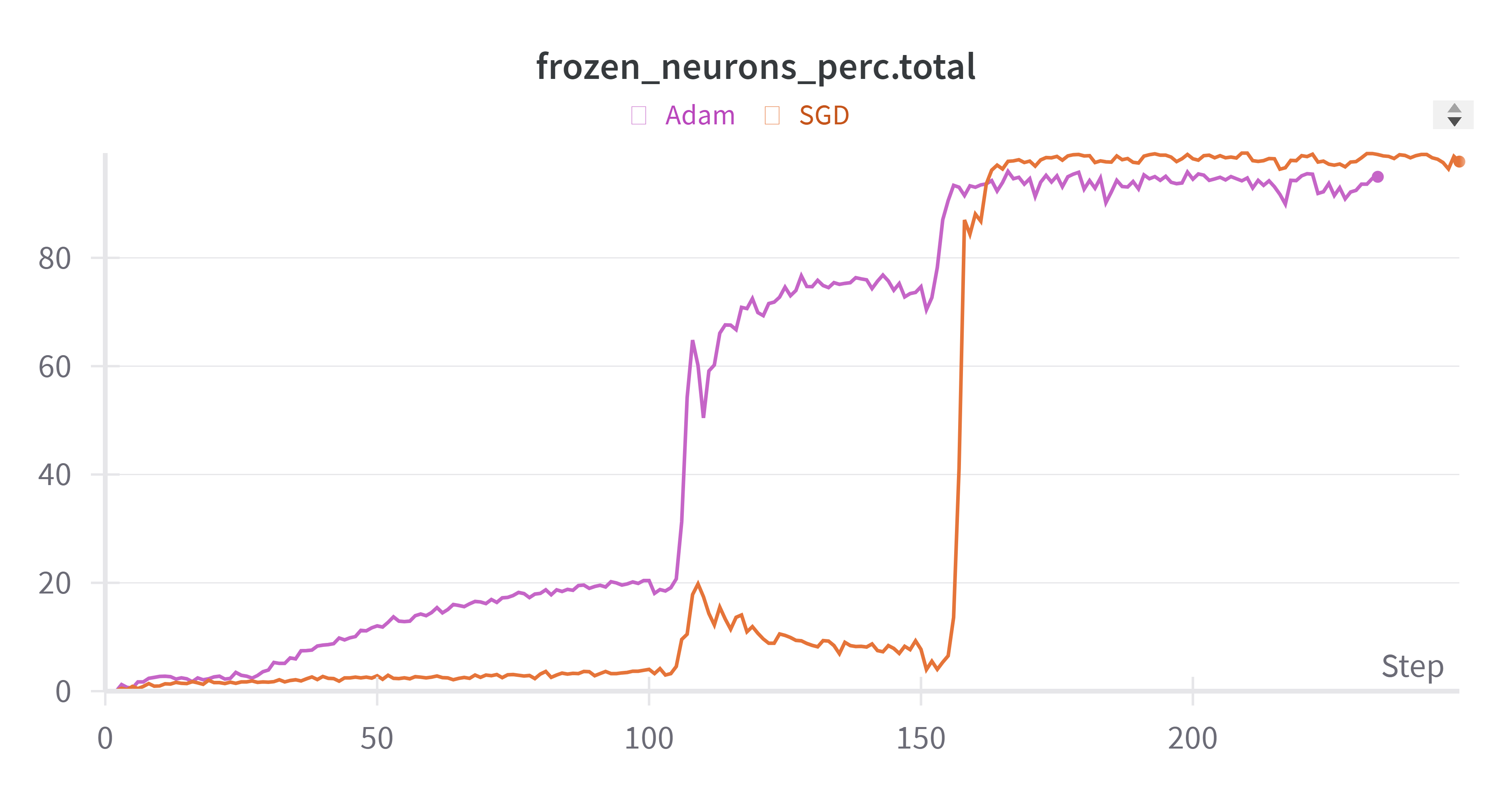
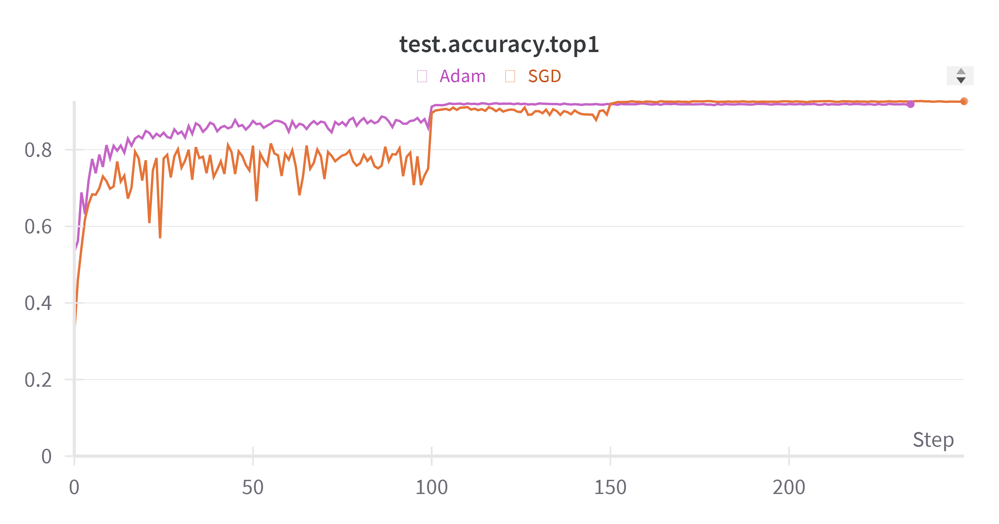
As expected, as training progresses and the learning rate is reduced, more neuron are frozen and the pattern found on the plot follow the one found by the authors with Adam freezing neuron faster than SGD. We also get the same accuracy level where Adam brings the network towards this equilibrium faster than SGD, but with SGD achieving a slightly higher final accuracy.
Conclusion
From the initial problem of computational resources saving, we have seen that NEq differs for others works that try to focus on finding optimal sub-graph for deep neural networks. By focusing on the entirety of the network and evaluating the behaviour of each neuron, NEq produces a new knowledge that is easily transposable to other experiments or any neural network model. The method results seem promising as it produces new insight on the learning behaviour of deep neural networks and might lead to new training strategies.
One possible development could be one of the limitations of the paper cited by the authors. The paper only focuses on individual neurons and evaluating the behaviour of ensembles of neurons could lead to other interesting results as some neurons might be at equilibrium only as a group at some step of the training process. This possibility could be explored further.
References
- Bragagnolo, A., Tartaglione, E., Grangetto, M.: To update or not to update? neurons at equilibrium in deep models. Advances in neural information processing systems, 2022.
- Dmitry Molchanov, Arsenii Ashukha, and Dmitry Vetrov. Variational dropout sparsifies deep neural networks. In International Conference on Machine Learning, pages 2498–2507. PMLR, 2017.
- J. Frankle and M. Carbin. The lottery ticket hypothesis: Finding sparse, trainable neural networks. 2019.