Learning Fair Scoring Functions: Bipartite Ranking under ROC-based Fairness Constraints
Learning Fair Scoring Functions: Bipartite Ranking under ROC-based Fairness Constraints
Authors: Godefroy LAMBERT and Louise DAVY
Table of Contents
- Introduction
- Definitions
- AUC-based fairness constraints
- ROC-based fairness constraints
- Results
- Reproducibility
- Conclusion
This is a blog post about the paper Learning Fair Scoring Functions: Bipartite Ranking under ROC-based Fairness Constraints, published by R. Vogel et al. in 2021 and available here.
Introduction
With recent advances in machine learning, applications are becoming increasingly numerous and the expectations are high. Those applications will only be able to be deployed if some important issues are addressed such as bias. There are famous datasets known for containing variables that induce a lot of bias such as Compas with racial bias and gender bias in the Adult dataset. To avoid those biases, new algorithms were created to provide more fairness in the prediction by using diverse methods.
Today, we will be reviewing the methods presented in “Learning Fair Scoring Functions: Bipartite Ranking under ROC-based Fairness Constraints”. This paper uses basic metrics such as AUC constraint and ROC constraint and shows some limitations. Since this is bipartite ranking, we will only focus on binary prediction, such as will this person recid for the COMPAS dataset or will this person get his loan for the Adult dataset.
Definitions
The goal of bipartite ranking is to acquire an ordering of X where positive instances are consistently ranked above negative ones with a high probability. This is done by learning an appropriate scoring function $s$. Such scoring functions are widely used in many critical domains such as loan granting, anomaly detection, or even in court decisions. A nice way to assess their performance is through the analysis of the Receiver Operating Characteristic (ROC) curve and the Area Under the ROC Curve (AUC).
ROC stands for Receiver Operating Characteristic curve and is a graph showing the performance of a classification model at all classification thresholds for a model. This curve plots two parameters:
- True Positive Rate
- False Positive Rate
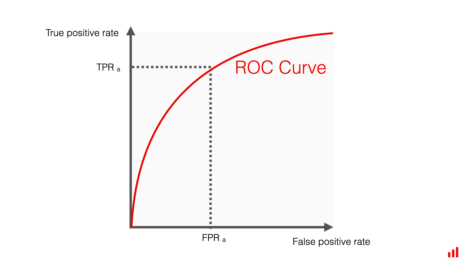
The formula for the True Positive Rate (TPR) is: $$TPR = \frac{TP}{TP + FN}$$
And the formula for the False Positive Rate (FPR) is: $$FPR = \frac{FP}{FP + TN}$$
With ${FP}$ = False Positive, $FN$ = False Negative, $TP$ = True Positive, $TN$ = True Negative.
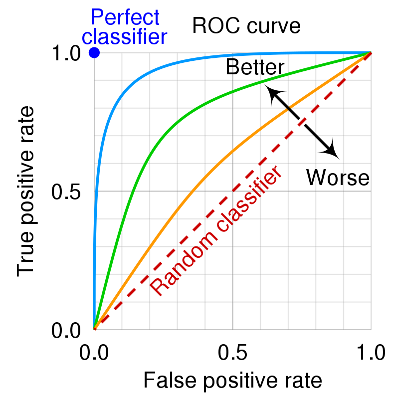
By varying the classifier, we can obtain different ROC curves that are represented in the following image. The curve that is closer to the upper-left corner is the best one, while the curve in diagonal represents a random classifier.
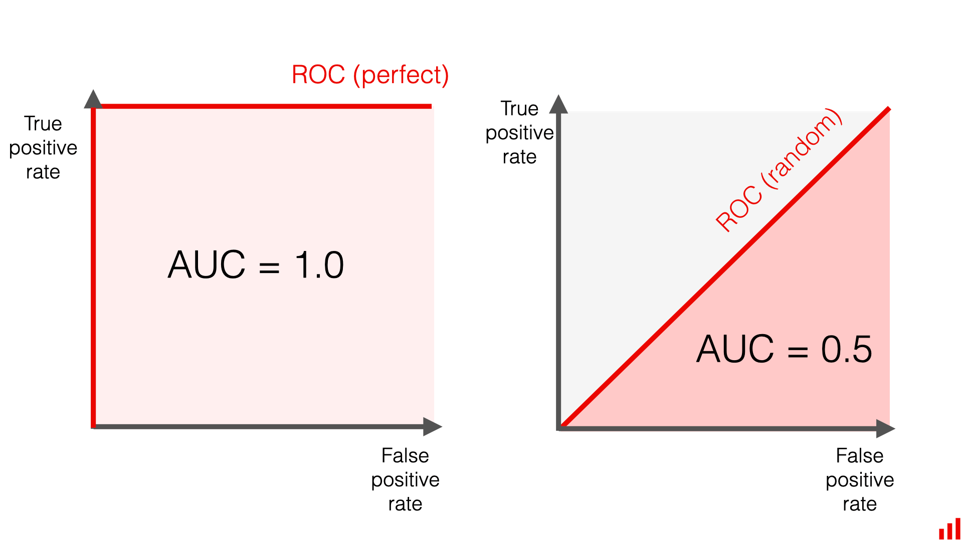
AUC stands for Area Under the ROC Curve and is a widely used metric in machine learning, particularly in binary classification tasks. The AUC quantifies the overall performance of the model across all possible classification thresholds.
That is, AUC measures the entire two-dimensional area underneath the entire ROC curve (think integral calculus) from (0,0) to (1,1). The AUC ranges in value from 0 to 1. A model whose predictions are 100% wrong has an AUC of 0.0, one whose predictions are 100% correct has an AUC of 1.0.
While fairness seems like a desirable goal for any ranking function, there are many different definitions of what fairness really is and thus, many different metrics to assess the fairness of an algorithm. In the case of loan grants for example, one could consider that fairness is achieved between men and women if we granted the same percentage of loans for both groups. Statistical parity, which compares the proportion of positive outcomes between different demographic groups, is a good metric in this case. However, this approach might overlook underlying disparities in socioeconomic status that affect loan approval rates. Another vision of fairness might ensure that individuals are all as likely to get a wrong decision, regardless of demographic factors such as gender or ethnicity. In this case, parity of mistreatment would be a good metric, as it ensures that the proportion of errors is the same for all demographic groups. However, this considers that all errors are the same, which means that one group could have a high false positive rate and another a high false negative rate. The authors thus decided to choose parity in false positive rates and/or parity in false negative rates.
AUC-based fairness constraints
This first approach is based on the AUC, it will help us to highlight the limitations of this metric which motivated the authors to introduce another approach based on ROC constraints.
Precise example of AUC based constraints presented in the paper are the intra-group pairwise AUC fairness (Beutel et al., 2019), Background Negative Subgroup Positive (BNSP) AUC fairness (Borkan et al., 2019), the inter-group pairwise AUC fairness (Kallus and Zhou, 2019). The first one require the ranking performance to be equal within groups, the second one enforces that positive instances from either group have the same probability of being ranked higher than a negative example and the last one imposes that the positives of a group can be distinguished from the negatives of the other group as effectively for both groups. Those 3 AUC based constraints are only a part of the many constraints that exist.
The paper introduces a new framework to generalize all relevant AUC-based constraint as a linear combination of 5 relevant elementary constraints noted $C_1$ to $C_5$.
The value of |$ C_ {1} $(s)| (resp. |$ C_ {2} $(s)|) quantifies the resemblance of the distribution of the negatives (resp. positives) between the two sensitive attributes.
$ C_ {1} $(s) = $ AUC_ {{H_S^{(0)}} ,{H_S^{(1)}}} $ - $\frac{1}{2}$
$ C_ {2} $(s) = $\frac{1}{2}$ - $ AUC_ {{G_S^{(0)}} ,{G_S^{(1)}}} $
The values of $ C_ {3} $(s), $ C_ {4} $(s) and $ C_ {5} $(s) measure the difference in ability of a score to discriminate between positives and negatives for any two pairs of sensitive attributes.
$ C_ {3} $(s) = $ AUC_ {{H_S^{(0)}} ,{G_S^{(0)}}} $ - $ AUC_ {{H_S^{(0)}} ,{G_S^{(1)}}} $
$ C_ {4} $(s) = $ AUC_ {{H_S^{(0)}} ,{G_S^{(1)}}} $ - $ AUC_ {{H_S^{(1)}} ,{G_S^{(0)}}} $
$ C_ {5} $(s) = $ AUC_ {{H_S^{(1)}} ,{G_S^{(0)}}} $ - $ AUC_ {{H_S^{(1)}} ,{G_S^{(1)}}} $
The family of fairness constraints considered is then the set of linear combinations of the $C_l(s)$ = 0:
\begin{align*} % $C_l(s)$ = 0 C_Γ(s): Γ^T C(s) = \sum_{l=1}^{5} {Γ_l}{C_l}(s) = 0 \end{align*}
Where $Γ$ = $(Γ_1, … Γ_5)^T$.
The objective function is thus defined as follows :
\begin{align} \label{eq:auc_general_problem} \textstyle\max_{s\in\mathcal{S}} \quad AUC_{H_s,G_s} - \lambda |\Gamma^\top C (s)|, \end{align} where $\lambda\ge 0$ is a hyperparameter balancing ranking performance and fairness.
The paper focuses on a special case of fairness, the intra-group pairwise AUC fairness. This was to be more concise. In this example, the objective function becomes:
$$ L_\lambda(s) = AUC_{H_s,G_s} - \lambda | AUC_{H_s^{(0)}, G_s^{(0)}} - AUC_{H_s^{(1)}, G_s^{(1)} } | $$
Issues of AUC-Based constraint:
Fairness using AUC-based constraints defined by the equality between two AUC’s only quantify a stochastic order between distributions, not the equality between these distributions, and would lead to some unfair result, for a group or for the other group.
The authors conducted experiments with the credit-risk dataset and found that creditworthy individuals from both groups had equal chances of being ranked higher than a “bad borrower.” However, employing high thresholds (which represent low probabilities of default on approved loans) would result in unfair outcomes for one group.
ROC-based fairness constraints
A richer approach is then to use pointwised ROC-based fairness constraints. Ideally, we would want to enforce the equality of all score distributions between both groups (i.e., identical ROC curves). This would satisfy all AUC-based fairness constraints previously mentioned. However, this condition is so restrictive that it will most likely lead to a significant drop in performances. As a result, the authors propose to satisfy this constraint on only a finite number of points. They were indeed able to prove that this was sufficient to ensure maximum fairness for a fixed false positive or false negative $\alpha$.
As a result, the objective function becomes :
\begin{align*} % L_\Lambda(s) = AUC_{H_s,G_s} &- \sum_{k=1}^{m_H} \lambda_H^{(k)} \big| \Delta_{H,\alpha_H^{ (k)}}(s) \big| - \sum_{k=1}^{m_G} \lambda_G^{(k)} \big| \Delta_{G,\alpha_G^{(k)}}(s) \big|, \end{align*}
Where $\Delta_{H,\alpha_H^{(k)}}(s)$ and $\Delta_{G,\alpha_G^{(k)}}(s)$ represent the deviations between the positive (resp. negative) inter-group ROCs and the identity function:
$$ \Delta_{G, \alpha}(s) = ROC_{G^{(0)}_s, G^{(1)}_s}(\alpha) - \alpha $$
$$ \Delta_{H, \alpha}(s) = ROC_{H^{(0)}_s,H^{(1)}_s}(\alpha) - \alpha $$
In practice, the objective function is slightly modified to be able to maximise it. The authors applied a classic smooth surrogate relaxations of the AUCs or ROCs based on a logistic function. They also removed the absolute values and, instead, relied on some parameters to ensure positive values.
Results
The authors tested out their results on two datasets : Compas and Adult. Both are widely used when it comes to fairness. Indeed, they are known to be biased against race (for Compas) and gender (for both). Compas is a recidivism prediction dataset, whereas Adult predicts whether income exceeds $50K/yr based on census data. The results reported in the next figure show that the ROC-based method achieves its goal of mitigating the differences between favoured and unfavoured groups with limited drop in performances (the AUC went from 0.72 to 0.70 on the Compas dataset and from 0.91 to 0.87 on the Adult dataset). Indeed, the blue ROC curve, which is the ROC curve of the unfavoured group (Afro-American people for the Compas Dataset and women for the Adult Dataset), is brought closer to the green ROC curve (the ROC curve of the favoured group).
Reproducibility
We were able to run the provided code without too much trouble on WSL2. The only modification we had to make was to change the calls for python in the sh files. We replace python with python3. However, as mentionned in the cide, the experiments were very long to run (several days) and we were not able to run the generate_all_figures.sh script fully as it made our computers crash. Still, we were able to get some of the figures found in the paper (see below) by launching some scripts separately.
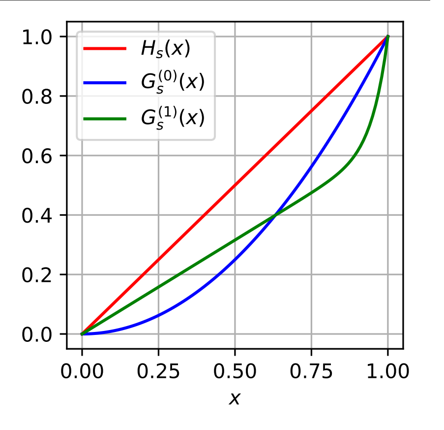
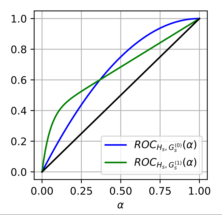
Here are two figure generated for the toy 1 dataset, one for the distribution of the scores and one for the ROC curve.
Conclusion
The paper “Learning Fair Scoring Functions: Bipartite Ranking under ROC-based Fairness Constraints” underscores the growing importance of fairness in machine learning applications. It shows the limits of AUC-based fairness constraints for their inability to ensure equality between distributions, potentially leading to unfair outcomes. In contrast, ROC-based fairness constraints offer a richer approach by enforcing equality of score distributions between groups, albeit with some performance trade-offs. The paper tests the method on typical fairness datasets, but it is also possible to apply it to reel use cases. “A Probabilistic Theory of Supervised Similarity Learning for Pointwise ROC Curve Optimization”, for example, explores the possibility to apply ROC-based methods for similarity learning, such as face recognition.
