Label-Free Explainability
Label-Free Explainability for Unsupervised Models
Authors: Valentina Hu and Selma Zarga
Table of Contents
This is a blog post about the paper Label-Free Explainability for Unsupervised Models, published by J. Crabbé et al. in 2022 and available here.
Why do we need explainability ?
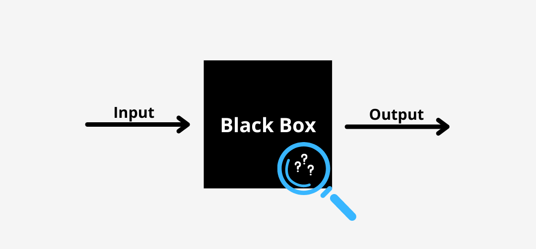
Machine learning models are becoming increasingly capable of making advanced predictions. While models like linear regression are relatively easy to understand and explain, more complex models, often called “black boxes” due to their complexity, present challenges in explaining how they make predictions. These models can be problematic in highstakes applications such as healthcare, finance, and justice, where it’s crucial to justify decision-making. Additionally, in case of errors, it’s important to understand the origin in order to address and correct them.
“Explainability is the cornerstone of trust in black box models; without it, they remain inscrutable and unreliable.” - Yoshua Bengio
To tackle this challenge, the field of Explainable Artificial Intelligence (XAI) has emerged, offering various methods to enhance model transparency. Post-Hoc explainability methods exist, which intervene after the model has generated its results, enabling users to comprehend the reasoning behind specific decisions or predictions. These methods supplement the predictions of black box models with diverse explanations of how they arrive at their predictions.

I. Introduction
The entire post focuses on the quest for explainability of unsupervised models. In these models, no labels are assigned to the data, making understanding the model even more complicated due to the absence of explicit guidance on what the model is learning. In the supervised setting, users know the meaning of the black-box output they are trying to interpret. However, this clarity is not always available in machine learning. Therefore, elucidating concepts such as feature importance and example importance provides insights into why the model makes certain decisions or identifies specific patterns in the data.
A recent research conducted by Crabbé and van der Schaar in 2022 explores the explainability of unsupervised models. They have developed two new methods to explain these complex models without labels. The first method highlights important features in the data, while the second identifies training examples that have the biggest impact on the model’s construction of representations. In this post, we will attempt to explain these two methods.
II. Feature Importance
Feature importance aims to explain how the model arrives at its prediction for a given input by assigning an importance scores to each feature (or attribute) of the input. This helps understand which features have the most influence on the model’s predictions. This method is developed based on a linear reasoning that is extended to label-free settings.
Given a model $( f : \mathcal{X} \rightarrow \mathcal{Y} )$, which maps an input space $( \mathcal{X} \subset \mathbb{R}^{d_X} )$ to an output space $( \mathcal{Y} \subset \mathbb{R}^{d_Y} )$. Where, $( d_X )$ and $( d_Y )$ is the dimensions of the input and output spaces.
In the traditionnal method, the process requires selecting one component $( f_j(x) )$ of the model’s output to compute the importance score for each feature $( i )$, denoted as $( a_i(f, x) )$. The selection is based on the ground-truth label, and $( j )$ corresponds to the class predicted with the highest probability.
To understand how the label-free feature importance method works, let’s start by looking at the labeled case:
1. Labelled Feature Importance
Authors introduces an alternative approach to calculate feature importance scores. The method proposes to combine the importance scores of different components of the model’s output by weighting them with the associated class probabilities. For each component of the model’s output, we multiply the importance score of the corresponding feature by the probability of that component.
These weighted importance scores are then combined to obtain the final importance score of each feature.
Let $a_i(f_j;x)$ be the importance score of feature $x_i$ calculated with respect to the component $f_j$ of the model’s output. The method proposes to calculate the importance score $b_i(f;x)$ for feature $x_i$ as follows:
$b_i(f;x) = \sum_{j=1}^{d_Y} f_j(x) \times a_i(f_j,x)$
Here, $f_j(x)$ represents the probability of class $j$, and $a_i(f_j;x)$ is the importance score of feature $x_i$ for class $j$.
Hovewer when the class probabilities are balanced, this method accounts for the contribution of each class to the feature importance score, rather than focusing only on the class with the highest probability, which is the usual practice.
This method proves to be efficient predominantly when the significance scores exhibit linearity in relation to the model. To facilitate a streamlined computation of weighted importance scores, another method is to introduce an auxiliary function, denoted as $(g_x)$ :
$\ g_x(z) = \sum_{j=1}^{d_Y} f_j(x) \cdot f_j(z) $
With the function $(g_x)$, it becomes feasible to calculate the weighted importance score, $(b_i(f, x))$, for each feature $(i)$, by merely employing $(g_x)$. This technique significantly simplifies the computational process, obviating the need to calculate $(d_Y \times d_X)$ importance scores. Such a calculation becomes impractically cumbersome with the escalation of the number of classes, $(d_Y)$. With this trick, we can compute the weighted importance score by only calling the auxiliary function.
We can see that in the labeled case, the method is quite clear. A similar reasoning is used in the label-free setting. Now, let’s move on to the label-free setting.
2. Label-Free Feature Importance
In the context of the unlabelled setting, we consider a latent space $H$ of dimension $d_H$ where a black-box model $f : X \rightarrow H$ is given. The goal is to assign an importance score to each feature of the input $x$, even if the dimensions of the latent space have no clear relations with the labels.
A similar weighting formula for importance scores is used, where the components $f_j(x)$ do not correspond to probabilities but to neuron activations. The weighted sum is considered as a inner product in the latent space.
The method is developed using linear feature importance functions, and it retains the completeness property, meaning that the sum of importance scores equals the black-box prediction up to a baseline constant.
Here is how the method operates:
Presentation of the Latent Space: We consider a latent space $H$ of dimension $d_H$ where each input $x$ is mapped by the black-box model $f$ to obtain a representation $h = f(x)$.
Assignment of Importance Scores: The objective is to assign an importance score $b_i(f; x)$ to each feature $x_i$ of $x$. Unlike in the previous setting, where we had probabilities associated with each component, here, we do not have a clear method to choose a particular component $f_j$ in the latent space. Therefore, we use a similar approach to the one described previously.
Calculation of Importance Scores: We use a weighting method where the importance score is given by $b_i(f; x) = a_i(\sum_{j=1}^{d_H} f_j(x) \cdot f_j(x))$. The individual components $f_j(x)$ do not correspond to probabilities in this case; they generally correspond to neuron activation functions. Inactive neurons will have a corresponding component that vanishes ($f_j(x) = 0$), meaning they will not contribute to the weighted sum, while more activated neurons will contribute more.
Completeness: An important property shared by many feature importance methods is completeness. This means that the sum of importance scores equals the black-box prediction up to a baseline constant. This establishes a connection between importance scores and black-box predictions.
This method proposes an extension of linear feature importance methods to the unlabelled setting by defining an auxiliary scalar function $g_x$ that encapsulates the black-box function $f$. This extension is achieved by using a function $g_x$ that computes the inner product between the representation $f(x)$ and the representation $f(\tilde{x})$ for all $\tilde{x}$ in the input space.
III. Example Importance
In this section, we explain the approach to extending example importance methods to the label-free setting. Given that example importance methods vary significantly, they are separated into two families: loss-based and representation-based methods. The extension to the label-free setting differs for these two families, so we discuss them separately in distinct subsections.
1. Loss-Based Example Importance
Supervised Setting
In supervised learning, loss-based example importance methods determine how important each training example is by assessing the impact of its removal on the model’s performance on test data. This is measured by the change in the loss function, which quantifies how well the model’s predictions match the true data.
Mathematically, let $z$ represent the data of an example required to evaluate the loss, typically corresponding to a pair $(x, y)$ in supervised settings. The loss function $L(z; \theta)$ is optimized over a parameter space $\Theta$ to train the model. When an example $z_n$ is removed from the training set $D_{\text{train}}$, it results in a parameter shift $\theta_n - \theta’_{-n}$, impacting the loss $L(z; \theta’)$ on a test example $z$. This loss shift provides a meaningful measure of example importance.
To estimate the loss shift without retraining the model, methods like the influence function and checkpoint evaluation are employed. For example, Koh & Liang (2017) propose using the influence function:
Influence Function Formula
\begin{equation} \langle
\delta_{\theta}^{n} L(z; \theta’) \approx \frac{1}{N} \langle {\nabla L(z; \theta_{*})}, H^{-1} {\nabla L(z_{n}; \theta_{*}’)} \rangle_{\theta}
\end{equation}
Where:
- $( \nabla_{\theta} L(z, \theta^*) )$ is the gradient of the loss with respect to the parameters for the test example.
- $( H_{\theta^*} )$ is the Hessian matrix.
- $( \nabla_{\theta} L(z^n, \theta^*) )$ is the gradient of the loss for the removed training example.
- $( \langle \cdot, \cdot \rangle_{\theta} )$ denotes the inner product in the parameter space.
- $( N )$ is the number of training examples.
Label-Free Setting
In a label-free setting, the models are trained without explicit labels. Instead, they use a label-free loss function, which typically tries to capture the structure of the data itself rather than fitting to specific target labels.
In the context of autoencoders, determining the importance of a training example can be tricky due to the loss function used during training (uses the encoder and decoder). When we are only interested in the encoder part and it is not sufficient to only use the model’s loss function as this also include the influence of the decoder.
To address this, we decompose the parameter space into relevant and irrelevant components. The proposed method computes the example importance scores by considering only the relevant parameters. The model to interpret, denoted as $f_r$, is parametrized only by the relevant parameters $\theta_r$.
This motivates the definition of Label-Free Loss-Based Example Importance:
\begin{equation} c_n(f_r; x) = \theta_n L(x; \theta’) \end{equation}
Label-Free Loss-Based Example Importance score $( c_n(f_{\theta_r}, x) )$ measures the impact of removing a training example $( x_n )$ from the training set on the learned latent representation $( f_{\theta_r}(x) )$ of a test example $( x )$. It uses $( \delta_{\theta_r} L )$ to denote the part of the loss shift that is only due to changes in the relevant parameters $(( \theta_r ))$.
This definition extends any loss-based example importance method to the label-free setting, where the unsupervised loss $L$ is used to fit the model, and the gradients with respect to the parameters of the encoder are computed.
2. Representation-Based Example Importance
Representation-based example importance methods analyze the latent representations of examples to assign importance scores.
Supervised Setting
These methods quantify the affinity between a test example and the training set examples based on their latent representations. For instance, in a model $f_l \circ f_e: X \rightarrow Y$, where $f_e: X \rightarrow H$ maps inputs to latent representations and $f_l: H \rightarrow Y$ maps representations to labels, representation-based methods reconstruct the test example’s latent representation using training representations. The reconstruction involves assigning weights to training representations, typically based on nearest neighbors or learned weights. For example, using a kernel function $\mathcal{K}$:
\begin{equation} w_n(x) = \frac{1}{|KNN(x)|} \sum_{n’ \in KNN(x)} \mathcal{K}(\text{fe}(x_n), \text{fe}(x)) \end{equation}
Label-Free Setting
Rrepresentation-based methods remain valid by replacing supervised representation maps with unsupervised ones. Hence, no additional modifications are needed.
IV. Experiments: Evaluation and Results
Consistency Checks
Now, we are verifying the consistency of results obtained from different methods of assessing feature and example importance using the MNIST dataset.
In MNIST, important features are the pixels of the images, and various methods can be employed to evaluate their importance. To assess feature importance, we can measure the impact of selectively removing the most important pixels on the latent representation constructed by the encoder, as described in the previous example. By comparing the results of different methods of importance assessment, such as perturbing the most important pixels according to various importance measures, we can check if the same pixels are identified as important and if their removal consistently affects the latent representation.
We rerun the tests provided in the GitHub repository:
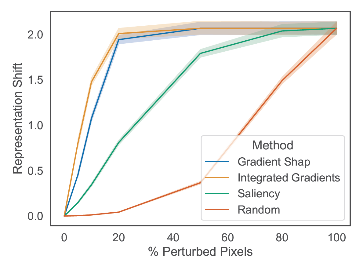
On the MNIST dataset, we perturb the most important pixels and observe how this perturbation affects the quality or relevance of the latent representation generated by the encoder. Here we can see the result of the experiment :

The results obtained from the representation shift curves as a function of the percentage of perturbed pixels demonstrate the effectiveness of Feature Importance methods on the MNIST dataset.
We observe that Feature Importance methods such as Gradient Shap and Integrated Gradients show a significant increase in representation shift when the most important pixels are perturbed. This indicates that these methods successfully identify the most relevant pixels for constructing the latent representation. However, after perturbing approximately 20% of the most important pixels, we notice a stabilization of the representation shift, suggesting that adding additional perturbations does not necessarily lead to a significant increase in impact on the latent representation.
On the other hand, the Saliency method appears to be less effective, with an almost linear representation shift curve, suggesting that it fails to selectively identify the most important pixels for the latent representation.
Overall, this confirms the effectiveness of Feature Importance methods, particularly Integrated Gradients.
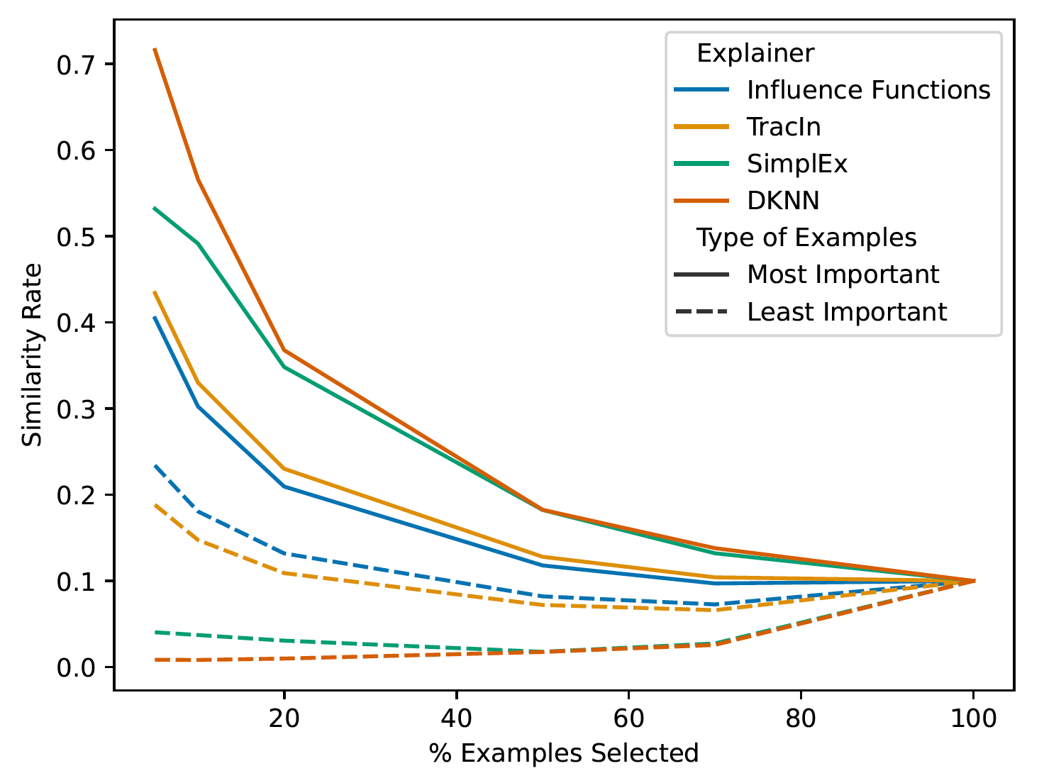
Similarly, to evaluate the importance of examples in MNIST, we select training examples that have a significant influence on predicting the latent representation of test examples. By comparing the results obtained with different methods of assessing example importance, we can verify if the same examples are identified as important and if their relevance is consistent with the model’s predictions.

For all example importance methods, we observe a decrease in similarity rates, with a consistent trend across all curves.
This observation highlights that the similarity rate is significantly higher among the most similar examples compared to the least similar examples, confirming the effectiveness of label-free importance scores cn(fe; x) in identifying training examples related to the test example we wish to explain.
In summary, these results affirm the capability of label-free importance scores in effectively selecting relevant training examples and distinguishing between similar and dissimilar examples.
V. Conclusion
In this post you learned about label-free explainability a new framework developped by Crabbé and van der Schaar in 2022, wich extend linear feature importance and example importance methods to the unsupervised setting with a focus on the MNIST dataset.
References
- Crabbé, J. & van der Schaar, M.. (2022). Label-Free Explainability for Unsupervised Models. Proceedings of the 39th International Conference on Machine Learning, in Proceedings of Machine Learning Research 162:4391-4420 Available from https://proceedings.mlr.press/v162/crabbe22a.html.