Knowledge Distillation: Boosting Interpretability in Deep Learning Models

Interpretability, the hidden power of knowledge distillation

Published March 15, 2025

bryanbradfo

Bryan Chen

remicsk

Rémi Calvet

Knowledge distillation is a powerful technique to transfer the knowledge from a large “teacher” model to a “student” model. While it’s commonly used to improve performance and reduce computational costs by compressing large models, this blog post explores a fascinating discovery: knowledge distillation can also enhance model interpretability. We’ll dive into the paper On the Impact of Knowledge Distillation for Model Interpretability" (ICML 2023) by H. Han et al., which sheds light on this novel perspective.

Interpretability in AI allows researchers, engineers, and decision-makers to trust and control machine learning models. Recent models show impressive performance on many different tasks and often rely on deep learning models. Unfortunately, deep learning models are also know for the difficulty to interprete them and understand how they come to a result wich can be problematic in highly sensitive applications like autonomous driving or healthcare. The article we present in this blog shows that knowledge distillation can improve the interpretability of deep learning models.

When AI is a black box, you’re just hoping for the best. But when you understand it, you become unstoppable.

0. Table of Contents

• I. Crash Course on Knowledge Distillation and Label Smoothing
• II. Defining Interpretability Through Network Dissection
• III. Logit Distillation & Feature Distillation: A Powerful Duo for Interpretability
• IV. Why Knowledge Distillation Enhances Interpretability
• V. Experimental Results and Reproduction
• VI. Beyond Network Dissection: Other Interpretability Metrics
• Conclusion
• Join the Discussion

I. Crash Course on Knowledge Distillation and Label Smoothing

What is Knowledge Distillation?

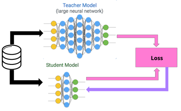
Knowledge distillation (KD) is a model compression technique introduced by Hinton et al. (2015) that transfers knowledge from a complex teacher model to a simpler student model. Unlike traditional training where models learn directly from hard labels (one-hot encodings), KD allows the student to learn from the teacher’s soft probability distributions.

The Key Mechanics of Knowledge Distillation

The standard KD loss function combines the standard cross-entropy loss with a distillation loss term:

$$\mathcal{L}_{KD}=(1-\alpha)\mathrm{CE}(y,\sigma(z_s))+\alpha T^2 \mathrm{CE}(\sigma(z_t^T),\sigma(z_s^T))$$

Where:

• $z_s$ and $z_t$ are the logits from the student and teacher models
• $T$ is the temperature parameter that controls softening of probability distributions
• $z_s^T \mathrel{:}= \frac{z_s}{T}$ and $z_t^T \mathrel{:}= \frac{z_t}{T}$
• $\sigma$ is the softmax function
• $\sigma(z_s^T) \mathrel{:}= \frac{\exp(z_s^T)}{\sum_j \exp(z_j^T)}$ and $\sigma(z_t^T) \mathrel{:}= \frac{\exp(z_t^T)}{\sum_j \exp(z_j^T)}$
• $\mathrm{CE}$ is cross-entropy loss
• $\alpha$ balances the importance of each loss component.

The first part of the loss $(1-\alpha)\mathrm{CE}(y,\sigma(z_s))$ is to incitate the student model to learn from one hot encoded ground truth label.

The second part of the loss $\alpha T^2 \mathrm{CE}(\sigma(z_t^T),\sigma(z_s^T))$ is to incitate the student model to try to reproduce the ouputs of the teacher model. This is what permits the student to learn from the teacher. The larger $\alpha$ is, the more the student will try to replicate the teacher model’s outputs and ignore the one hot encoded groundtruth and vice versa.

Label Smoothing

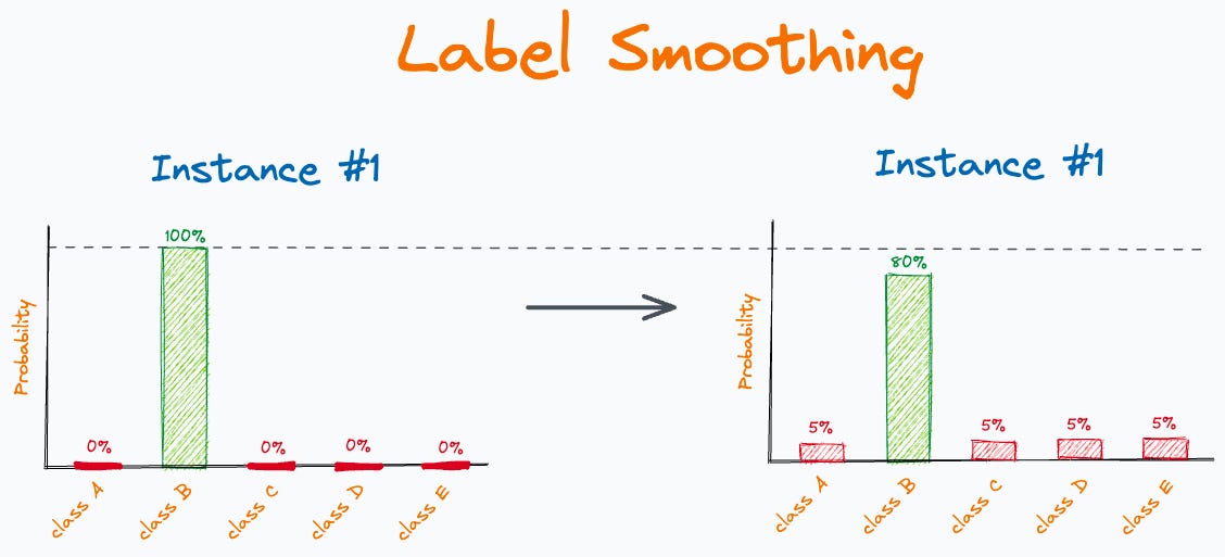
Label smoothing (LS) is another technique that smooths hard targets by mixing them with a uniform distribution. In the cross entropy loss we replace the one hot encoded $y$ by $y_{LS} \mathrel{:}= (1-\alpha)y + \frac{\alpha}{K}$, where $K$ is the number of classes and $\alpha$ the smoothing parameter:

We obtain a loss that is similar to knowledge diffusion but there is a key difference important for interpretability that we will discuss later. From the equation above, we get the label smoothing loss equation: $$L_{LS} = (1-\alpha)\mathrm{CE}(y,\sigma(z)) + \alpha\mathrm{CE}(u,\sigma(z)) $$ Where $u$ is a uniform distribution over all the possible $K$ classes.

II. Defining Interpretability Through Network Dissection

The first thing to know is that there are different approaches to define and measure interpretability in machine learning.

For image classification, the authors use network dissection to quantitatively measure interpretability. The idea is to compare activation maps and see if areas with high activation correspond to an object or a meaningful concept on the image.

The process can be better understood through the following illustration:

Feed a neural network model an image, pick a deep layer and count the number of neurons that detects a concept like “cat” or “dog”. We call those neurons concept detectors and will define them more precisely. The number of concept detectors will be the primary metric to define the interpretability of a model, the higher the more we will consider it interpretable.

The easiest way to understand what is a concept detector is to look at the following pseudo code to compute the number of concept detectors:

If you prefer to understand with code, here is an implementation of the procedure described above:

def identify_concept_detectors(model, layer_name, dataset, concept_masks):
    """
    Identify neurons that act as concept detectors in a specific layer.

    Args:
        model: Neural network model
        layer_name: Name of the layer to analyze
        dataset: Dataset with images
        concept_masks: Dictionary mapping images to concept segmentation masks

    Returns:
        Dictionary mapping neurons to detected concepts
    """
    # Step 1: Collect activation maps for each image
    activation_maps = {}

    for image in dataset:
        # Forward pass and extract activation at specified layer
        activations = get_layer_activation(model, layer_name, image)

        for neuron_idx, activation in enumerate(activations):
            if neuron_idx not in activation_maps:
                activation_maps[neuron_idx] = []
            activation_maps[neuron_idx].append(activation)

    # Step 2: Compute threshold for top 0.5% activations for each neuron
    thresholds = {}
    for neuron_idx, activations in activation_maps.items():
        # Flatten all activations for this neuron
        all_activations = torch.cat([act.flatten() for act in activations])
        # Compute threshold for top 0.5%
        threshold = torch.quantile(all_activations, 0.995)
        thresholds[neuron_idx] = threshold

    # Step 3: Create binary masks and compute IoU with concept masks
    concept_detectors = {}

    for image_idx, image in enumerate(dataset):
        image_concepts = concept_masks[image_idx]

        for neuron_idx, activations in activation_maps.items():
            # Get activation for this neuron on this image
            activation = activations[image_idx]

            # Create binary mask using threshold
            binary_mask = (activation >= thresholds[neuron_idx]).float()

            # Resize to match image dimensions
            binary_mask = F.interpolate(
                binary_mask.unsqueeze(0).unsqueeze(0),
                size=image.shape[1:],
                mode='bilinear'
            ).squeeze()

            # Compute IoU with each concept mask
            for concept, mask in image_concepts.items():
                intersection = torch.sum(binary_mask * mask)
                union = torch.sum(binary_mask) + torch.sum(mask) - intersection
                iou = intersection / union if union > 0 else 0

                # If IoU exceeds threshold (typically 0.05), consider it a detector
                if iou > 0.05:
                    if neuron_idx not in concept_detectors:
                        concept_detectors[neuron_idx] = set()
                    concept_detectors[neuron_idx].add(concept)

    return concept_detectors

III. Logit Distillation & Feature Distillation: A Powerful Duo for Interpretability

Combining logit distillation with feature distillation not only boosts performance but also enhances the interpretability of student models. This improvement is measured by an increase in the number of concept detectors, which represent units aligned with human-interpretable concepts.

where Attention Transfer (AT), Factor Transfer (FT), Contrastive Representation Distillation (CRD), and Self-Supervised Knowledge Distillation (SSKD) are all variations of knowledge distillation techniques, each designed to transfer knowledge from teacher models to student models in unique ways.

How they work together?

1. Logit Distillation:

• Transfers class-similarity information from the teacher to the student through softened logits.
• Helps the student model understand the relationships between semantically similar classes, making activation maps more object-centric.

2. Feature Distillation:

• Focuses on aligning intermediate layer features between the teacher and student.
• Improves the student model’s ability to replicate the teacher’s feature representations, supporting richer internal representations.

IV. Why Knowledge Distillation Enhances Interpretability

The key insight from the paper is that knowledge distillation transfers not just the ability to classify correctly, but also class-similarity information that makes the model focus on more interpretable features.

Transfer of Class Similarities

When a teacher model sees an image of a dog, it might assign:

• 85% probability to “Golden Retriever”
• 10% probability to other dog breeds
• 5% probability to other animals and objects

These “soft targets” (consequence of logit distillation) encode rich hierarchical information about how classes relate. The student model distilling this knowledge learns to focus on features that are common to similar classes (e.g., general “dog” features).

Label Smoothing vs. Knowledge Distillation

By looking at the KD and label smoothing losses, we can see that they are similar. When $T=1$ they only differ in the second member where we have a $\sigma(z_t^T)$ that contains class-similarity information instead of $u$ that doesn’t contain any information.

• $\mathcal{L}_{KD}=(1-\alpha)\mathrm{CE}(y,\sigma(z_s))+\alpha T^2 \mathrm{CE}(\sigma(z_t^T),\sigma(z_s^T))$
• $L_{LS} = (1-\alpha)\mathrm{CE}(y,\sigma(z)) + \alpha\mathrm{CE}(u,\sigma(z)) $

So, if there is a difference in interpretability, it is likely that it comes from the fact that distillation permits to get class similarity knowledge from the teacher model. This is exactly what is shown in the figure below. Knowledge distillation guides student models to focus on more object-centric features rather than background or contextual features. This results in activation maps that better align with the actual objects in images.

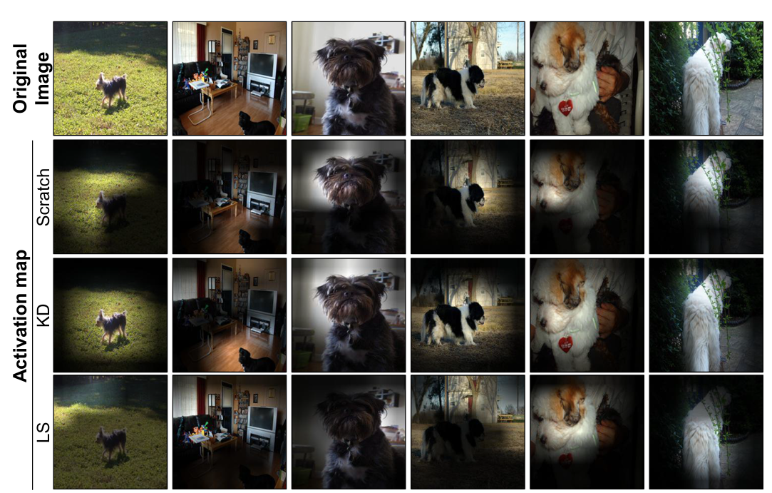
The next figure also highlights the loss of interpretability (less concept detectors) when using label smoothing and the improvement of interpretability (more concept detectors) for KD:

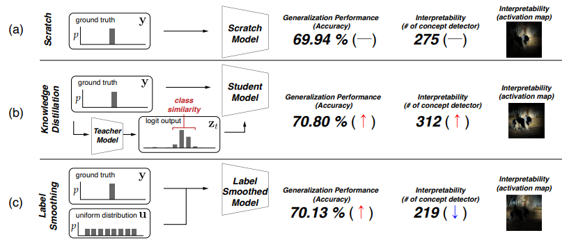
While label smoothing can improve accuracy, it often reduces interpretability by erasing valuable class relationships while KD keeps class relationship information and improves both accuracy and interpretability.

V. Experimental Results and Reproduction

Let’s implement a reproduction of one of the paper’s key experiments to see knowledge distillation’s effect on interpretability in action.

Setting Up the Experiment

We are going to replicate the experiment by using the GitHub repository provided by the authors. The repository contains the code to train the models, compute the concept detectors, and evaluate the interpretability of the models.

As it is often the case with a machine learning paper, running the code to reproduce results requires some struggle. To reproduce the results, you could use a virtual environment (e.g. SSP Cloud Datalab) and then do the following:

git clone https://github.com/Rok07/KD_XAI.git
cd torchdistill
pip install -e .
cd ..
bash script/dlbroden.sh
nano torchdistill/torchdistill/models/custom/bottleneck/__init__.py
~ comment the first line
pip install opencv-python
pip install imageio
sudo apt update
sudo apt install -y libgl1-mesa-glx
nano util/vecquantile.py
~ change NaN by nan
nano loader/data_loader.py
~ add out[i] = rgb[:,:,0] + (rgb[:,:,1].astype(np.uint16) * 256)
cd ..
nano settings.py
~ change TEST_MODE = False to True
cd dataset/broden1_224
cp index.csv index_sm.csv
~ keep the 4000 first lines
cd ../..
nano visualize/bargraph.py
~ change parameter threshold of bar_graph_svg() to 0.001
python main.py

Network Dissection quantifies the interpretability of hidden units by measuring their alignment with human-interpretable concepts. The following results reveal several interesting findings:

1. Concept Distribution (from bargraph.svg):

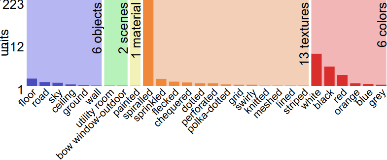
• ~6 units detecting object concepts
• ~2 units detecting scene concepts
• 1 unit detecting material properties
• ~13 units detecting textures
• ~6 units detecting colors

2. Specific Units: (layer4-0xxx.jpg)

• Unit 330 has specialized in detecting grid and regular pattern textures

• Unit 202 detects sky regions in images

The network dissection approach reveals interpretable neurons of a distilled ResNet18.

VI. Beyond Network Dissection: Other Interpretability Metrics

While the paper emphasizes the use of Network Dissection to measure model interpretability by quantifying concept detectors, it also explores several additional metrics to confirm the broader impact of Knowledge Distillation (KD) on interpretability:

• Five-Band Scores, proposed by Tjoah & Guan (2020): This metric assesses interpretability by evaluating pixel accuracy (accuracy of saliency maps in identifying critical features), precision (how well the saliency maps match the actual distinguishing features), recall, and false positive rates (FPR, lower FPR indicates better interpretability) using a synthesized dataset with heatmap ground truths. KD-trained models consistently show higher accuracy and lower FPR compared to other methods.
• DiffROAR Scores, proposed by Shah et al. (2021): This evaluates the difference in predictive power on a model trained on a dataset and a model trained on a version of the dataset where we removed top and bottom x% of the pixel according to their importance for the task. The authors find that KD has a higher DiffROAR score than a model trained from scratch. It means that KD makes the model use more relevant features and thus more interpretable in that sense.
• Loss Gradient Alignment: This metric measures the alignment of model gradients with human-perceived important features. KD models exhibit better alignment, indicating greater interpretability as we can see on this figure:

  

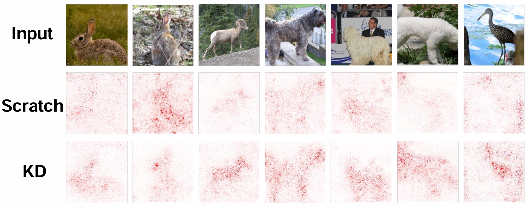
These metrics collectively show that KD can enhance interpretability. The consistent results showing that knowledge distillation can enhance interpretability for different metrics of interpretability provide strong arguments to believe that KD could be broadly used for better interpretability of deep learning models.

Conclusion

The article showed that knowledge distillation can improve both accuracy and interpretability. They attribute the improvement in interpretability to the transfer of class similarity knowledge from the teacher to the student model. They compare label smoothing (LS) that is similar to KD but LS does not benefit from class-similarity information. The empirical experiments shows better accuracy for LS and KD but the interpretability of LS decreases whereas it increases for KD confirming the hypothesis that class similarity knowledge has a role in interpretability. The authors obtain consistent results when using other metrics than the number of concept detectors for interpretability showing that their approach is robust to different definitions of interpretability.

Those encouraging results could lead to applications of knowledge distillation to improve the interpretability of deep learning models in highly sensitive areas like autonomous systems and healthcare.

Join the Discussion

We’d love to hear your thoughts! What are your experiences with Knowledge Distillation (KD)? Have you found it to improve not just performance but also interpretability in your projects? Feel free to share your ideas, questions, or insights in the comments section or engage with us on GitHub!

References

• Hinton, G., Vinyals, O., & Dean, J. (2015). Distilling the knowledge in a neural network. arXiv:1503.02531.
• Han, H., Kim, S., Choi, H.-S., & Yoon, S. (2023). On the Impact of Knowledge Distillation for Model Interpretability. arXiv:2305.15734.
• Bau, D., Zhou, B., Khosla, A., Oliva, A., & Torralba, A. (2017). Network dissection: Quantifying interpretability of deep visual representations. arXiv:1704.05796.
• Tjoa, E., & Guan, M. Y. (2020). Quantifying explainability of saliency methods in deep neural networks. arXiv:2009.02899.
• Shah, H., Jain, P., & Netrapalli, P. (2021). Do input gradients highlight discriminative features? arXiv:2102.12781, NeurIPS 2021.