A Framework to Learn with Interpretation
A Framework to Learn with Interpretation
Authors: Maroun ABOU BOUTROS, Mohamad EL OSMAN
Article: A Framework to Learn with Interpretation by Jayneel Parekh, Pavlo Mozharovskyi and Florence d’Alché-Buc
Table of Contents
- Introduction
- Learning a classifier and an interpreter
- Understanding encoded concepts in FLINT
- Reproducing the experiments
- Subjective evaluation
- Specialization of FLINT to post-hoc interpretability
- Conclusion
1 Introduction
In this blog post, we’ll explore FLINT, a framework introduced in the paper titled “A Framework to Learn with Interpretation” by Jayneel Parekh, Pavlo Mozharovskyi and Florence d’Alché-Buc, available on the following link, addressing the crucial need for interpretability in machine learning as complex predictive models become more prevalent in fields like law, healthcare, and defense. Interpretability, synonymous with explainability, provides insights into a model’s decision-making process. Two main approaches, post-hoc methods and “interpretable by design” methods, tackle the challenge of interpreting models, each with its pros and cons. A new approach, Supervised Learning with Interpretation (SLI), jointly learns a predictive model and an interpreter model. FLINT, specifically designed for deep neural network classifiers, introduces a novel interpreter network architecture promoting local and global interpretability. It also proposes a criterion for concise and diverse attribute functions, enhancing interpretability. We’ll delve into the architecture of FLINT and how it works to give explainable predictions, and we will reproduce some experiments done in the experimental section of the article and evaluate their outputs to study FLINT’s performance. And finally, we will present a specialization of FLINT for post-hoc interpretability.
2 Learning a classifier and its interpreter with FLINT
The paper introduces Supervised Learning with Interpretation (SLI), a new task aimed at incorporating interpretability alongside prediction in machine learning models. In SLI, a separate model, called an interpreter, is employed to interpret the predictions made by the primary predictive model. The task involves minimizing a combined loss function consisting of prediction error and interpretability objectives. The paper focuses on addressing SLI within the context of deep neural networks for multi-class classification tasks. It proposes a framework called Framework to Learn with INTerpretation (FLINT), which utilizes a specialized architecture for the interpreter model, distinguishes between local and global interpretations, and introduces corresponding penalties in the loss function to achieve the desired interpretability.
So for a dataset $S$ and a given model $f \in F$ where $F$ is a class of classifiers (here neural networks) and an interpreter model $g \in G_f$ where $G_f$ is a family of models, the SLI problem is presented by:
$$
\arg{\min_{f \in F, g \in G_f}{L_{pred}(f, S) + L_{int}(f, g, S)}}
$$
Where $L_{pred}(f, S)$ denotes a loss term related to prediction error and $L_{int}(f, g, S)$ measures the ability of $g$ to provide interpretations of predictions by $f$.
2.1 Design of FLINT

In FLINT, depicted in the image above, both a prediction model ($f$) and an interpreter model ($g$) are used. The input to FLINT is a vector $x \in X$, where $X = \mathbb{R}^d$, and the output is a vector $y \in Y$, where $Y$ is defined as the set of one-hot encoding vectors with binary components of size $C$ (the number of classes to predict). The prediction model $f$ is structured as a deep neural network with $l$ hidden layers, represented as $f = f_{l+1} \circ f_l \circ \ldots \circ f_1$. Each $f_k$ represents a hidden layer mapping from $R^{d_{k-1}}$ to $R^{d_k}$. To interpret the outputs of $f$, we randomly select a subset of $T$ hidden layers, indexed by $I=\{i_1, i_2, \ldots, i_T\}$, and concatenate their outputs to form a new vector $f_I(x) \in \mathbb{R}^D$, where $D = \sum_{t=1}^T d_{i_t}$. This vector is then fed into a neural network $\Psi$ to produce an output vector $\Phi(x) = \Psi(f_I(x)) = (\phi_1(x), …, \phi_J (x)) \in \mathbb{R}^J$, representing an attribute dictionary comprising functions $\phi_j: X \rightarrow \mathbb{R}^+$, where $\phi_j(x)$ captures the activation of a high-level attribute or a “concept” over $X$. Finally, $g$ computes the composition of the attribute dictionnary with an interpretable function $h: R^J \rightarrow Y$. $$ \forall x \in X, g(x) = h(\Phi(x)) $$ For now we take $h(x) = softmax(W^T \Phi(x))$ but $h$ can be any interpretable function (like a decision tree for example).
Note that $d$ in the image is a decoder network that takes $\Phi(x)$ and reconstructs the input $x$. This decoder is used for training and its purpose will be detailed later on in section 2.3.
2.2 Interpretation in FLINT
With the interpreter defined, let’s clarify its role and interpretability objectives within FLINT. Interpretation serves as an additional task alongside prediction. We’re interested in two types: global interpretation, which aids in understanding which attribute functions contribute to predicting a class, and local interpretation, which pinpoints the attribute functions involved in predicting a specific sample.
To interpret a local prediction $f(x)$, it’s crucial that the interpreter’s output $g(x)$ aligns with $f(x)$. Any discrepancy prompts analysis of conflicting data, potentially raising concerns about the prediction’s confidence.
To establish local and global interpretation, we rely on attribute relevance. Given an interpreter with parameters $\Theta_g = (\theta_\Psi, \theta_h)$ and an input $x$, an attribute $\phi_j$’s relevance is defined concerning the prediction $g(x) = f(x) = \hat{y}$. The attribute’s contribution to the unnormalized score of class $\hat{y}$ is $\alpha_{j, \hat{y}, x} = \phi_j(x) \cdot w_{j, \hat{y}}$, where $w_{j, \hat{y}}$ is the coefficient associated with this class. Relevance score $r_{j, x}$ is computed by normalizing $\alpha$ as $r_{j, x} = \frac{\alpha_{j, \hat{y}, x}}{\max_i |\alpha_{i, \hat{y}, x}|}$. An attribute $\phi_j$ is considered relevant for a local prediction if it’s both activated and effectively used in the linear model.
Attribute relevance extends to its overall importance in predicting any class $c$. This is achieved by averaging relevance scores from local interpretations over a random subset or the entirety of the training set $S$ where the predicted class is $c$. Thus, $r_{j, c} = \frac{1}{|S_c|} \sum_{x \in S_c} r_{j, x}$, where $S_c = \{x \in S \mid \hat{y} = c\}$.
Now, let’s introduce the local and global interpretations the interpreter will provide:
Global interpretation ($G(g, f)$) identifies class-attribute pairs $(c, \phi_j)$ where the global relevance $r_{j, c}$ exceeds a threshold $\frac{1}{\tau}$.
Local interpretation ($L(x, g, f)$) for a sample $x$ includes attribute functions $\phi_j$ with local relevance $r_{j, x}$ surpassing $\frac{1}{\tau}$. These definitions don’t assess interpretation quality directly.
2.3 Learning by imposing interpretability properties
For learning, the paper defines certain penalties to minimize, where each one aims to enforce a certain desirable property:
Fidelity to output: The output of $g(x)=h(\Psi(f_I(x)))$ should be close to $f(x)$ for any x. This can be imposed through a cross-entropy loss: $$ L_{of}(f, g, S) = - \sum_{x \in S} h(\Psi(f_I(x)))^T \log(f(x)) $$
Conciseness and Diversity of Interpretations: We aim for concise local interpretations, containing only essential attributes per sample, promoting clearer understanding and capturing high-level concepts. Simultaneously, we seek diverse interpretations across samples to prevent attribute functions from being class-exclusive. To achieve this, the paper proposes that we leverage entropy (defined for a vector as $\mathcal{E}(v) = - \sum_i p_i \log(p_i)$), which quantifies uncertainty in real vectors. Conciseness is fostered by minimizing the entropy of the interpreter’s output, $\Phi(x) = \Psi(f_I(x))$, while diversity is encouraged by maximizing the entropy of the average $\Psi(f_I(x))$ over a mini-batch. This approach promotes sparse and varied coding of $f_I(x)$, enhancing interpretability. However, as entropy-based losses lack attribute activation constraints, leading to suboptimal optimization, we also minimize the $l_1$ norm of $\Psi(f_I(x))$ with hyperparameter $\eta$. Although $l_1$-regularization commonly encourages sparsity, the experiments done in the paper show that entropy-based methods are more effective. $$ L_{cd}(f, g, S) = -\mathcal{E}(\frac{1}{\lvert S \lvert} \sum_{x \in S} \Psi(f_I(x))) + \sum_{x \in S} \mathcal{E}(\Psi(f_I(x))) + \sum_{x \in S} \eta \lVert \Psi(f_I(x)) \lVert_1 $$
Fidelity to input: In order to promote the representation of intricate patterns associated with the input within $\Phi(x)$, a decoder network $d : \mathbb{R}^J \rightarrow X$ is employed. This network is designed to take the attribute dictionary $\Phi(x)=\Psi(f_I(x))$ as input and reconstruct the original input $x$. $$ L_{if}(f, g, d, S) = \sum_{x \in S} (d(\Psi(f_I(x))) - x)^2 $$
Given the proposed loss terms, the loss for the interpretability model writes as follows: $$ L_{int}(f, g, d, S) = \beta L_{of}(f, g, S) + \gamma L_{if}(f, g, d, S) + \delta L_{cd}(f, g, S) $$ Where $\beta, \gamma, \delta$ are non-negative hyperparameters. the total loss to be minimized $L = L_{pred} + L_{int}$, where the prediction loss, $L_{pred}$, is the well-know cross entropy loss (since this a classification problem).
3 Understanding encoded concepts in FLINT
Once the predictor and interpreter networks are jointly learned, interpretation can be conducted at both global and local levels . A critical aspect highlighted by the authors is understanding the concepts encoded by each individual attribute function $\phi_j$ . Focusing on image classification, the authors propose representing an encoded concept as a collection of visual patterns in the input space that strongly activate $\phi_j$ . They present a pipeline for generating visualizations for both global and local interpretation, adapting various existing tools .
For global interpretation visualization, the authors propose starting by selecting a small subset of training samples from a given class c that maximally activate $\phi_j$ . This subset, referred to as Maximum Activating Samples (MAS), is denoted as $MAS(c , \phi_j , l)$ where $l$ is the subset size (set as 3 in their experiments). However, while MAS provides some insight into the encoded concept, further analysis is required to understand the specific aspects of these samples that cause $\phi_j$ activation. To achieve this, the authors propose utilizing a modified version of activation maximization called Activation Maximization with Partial Initialization (AM+PI). This technique aims to synthesize input that maximally activates $\phi_j$ by optimizing a common activation maximization objective, initialized with a low-intensity version of the sample from MAS.
For local analysis, given any test sample $x_{0}$ , its local interpretation $L(x_{0},f,g)$ can be determined, representing the relevant attribute functions . To visualize a relevant attribute $\phi_j$, the authors suggest repeating the AM+PI procedure with initialization using a low-intensity version of $x_{0}$ to enhance the concept detected by $\phi_j$ in $x_{0}$ .
4 Reproducing the experiments
In the experimental section of the article, several experiments were conducted to do a quantitative evaluation of FLINT’s performance compared to other state-of-the-art models designed for interpretability, such as SENN and PrototypeDNN. Additionally, FLINT was compared to LIME and VIBI to evaluate the fidelity of its interpretations, measuring the proportion of samples where the predictions of a model and its interpreter agree. Across these tests, FLINT consistently outperformed the other models, demonstrating its reliability and effectiveness.
However, in this blog post we will specifically focus on reproducing the experiments in the article related to FLINT’s explainability, that aim to do a qualitative analysis of it. To achieve a thorough understanding of the model and its operational dynamics across prevalent datasets, we replicated the study by cloning the project from the GitHub repository referenced in the article (repo link). Our experimentation involved the CIFAR10 and QuickDRAW datasets, employing a ResNet18-based network for both. For the QuickDRAW dataset, we utilized J=24 attributes, while for the CIFAR10 dataset, we used J=36 attributes.
The instructions provided in the GitHub repository for executing the model are clear, and the model runs flawlessly. We have the option to either train the model ourselves or download the pre-trained models. Furthermore, there is a well-detailed Python notebook named “FLINT demo.ipynb”, which contains code for visualizing data, such as attribute relevance scores for each class and local interpretations for data samples. We will execute FLINT on test images and take a look at how interpretability is done with FLINT in this section.
4.1 Global interpretation
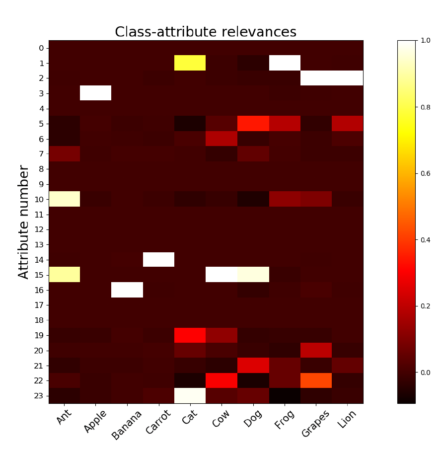
In the article, the authors explore global interpretation using a figure similar to the one provided below which was reproduced from the notebook, and which illustrates the generated global relevances $r_{j,c}$ for all class-attribute pairs in the QuickDraw dataset.

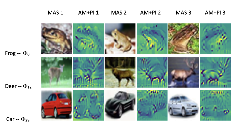
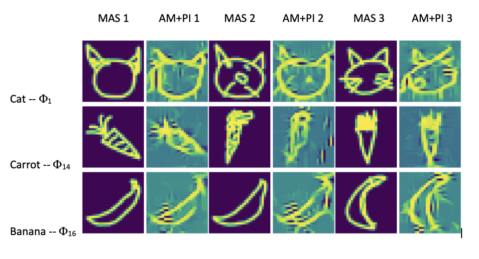
Additionally, by running the model on the CIFAR10 and QuickDRAW dataset we got visual outputs representative of class-attribute pair analyses for both datasets. These outputs served as pivotal tools in elucidating interrelations and facilitating comparative assessments between attributes and classes. We present below two figures derived from the resultant class-attribute pair analyses for each of the 2 datasets. The class-attribute pairs shown are different from the examples shown in the paper.
 Caption: Class-attribute pair analysis on dataset CIFAR10
 Caption: Class-attribute pair analysis on dataset QuickDraw
We focus on class-attribute pairs with high relevance, showcasing examples in the provided figure above . For each pair, we examine Maximum Activating Samples (MAS) alongside their corresponding Activation Maximization with Partial Initialization (AM+PI) outputs.
MAS analysis alone provides valuable insights into the encoded concept. For instance, on QuickDRAW dataset, attribute $\phi_{16}$ relevant for class ‘Banana’ activates the curve shape of the banana. However, AM+PI outputs offer deeper insights by elucidating which parts of the input activate an attribute function more clearly. And on CIFAR10 dataset , attribute $\phi_{12}$ activates for ‘Deer’ class , but the specific focus of the attribute remains ambiguous. The outputs of the AM+PI method indicate that attribute $\phi_{12}$ predominantly highlights the area encompassing the legs and the horns of the deer, characterized as the most prominently enhanced regions.
4.2 Local interpretation
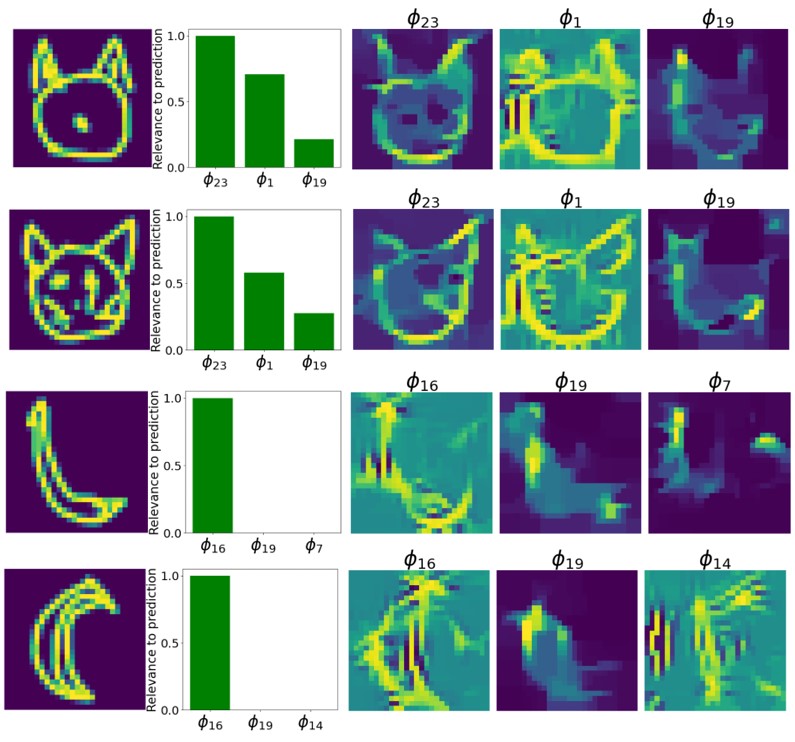
Similarly to the article, we explored local interpretation through the figure provided below which was generated in the notebook, which showcases visualizations for 4 test samples of the QuickDRAW dataset. Both predictor $f$ and interpreter $g$ accurately predict the true class in all cases, for the first 2 it’s “Cat” and the last 2 it’s “Banana”. For each case, they highlighted the top 3 relevant attributes to the prediction along with their relevances and corresponding AM+PI outputs.

Analysis of the AM+PI outputs reveals that attribute functions generally activate for patterns corresponding to the same concept inferred during global analysis. This consistency is evident for attribute functions present in the previous figures. Additionaly, by looking at the figure showing the relevance of class-attribute pairs in section 4.1 for the QuickDRAW dataset we observe that the 3 most important features for each class in the local interpretations are also those having the highest relevence for these classes. For example for the “Banana” class, $\phi_{16}$, which activates the curve shape, is by far the most important feature for identifying this class by looking at both the local interpretations and the class-attribute relevences. While for the “Cat” class, it seems that the most important features are in order $\phi_{23}$, $\phi_1$ and $\phi_{19}$ when looking at both the local interpretations and the class-attribute relevences.
5 Subjective evaluation
In the article, a subjective evaluation survey with 20 respondents using the QuickDraw dataset to assess FLINT’s interpretability is conducted. The authors selected 10 attributes covering 17 class-attribute pairs and presented visualizations (3 MAS and AM+PI outputs) along with textual descriptions for each attribute to the respondents. They were asked to indicate their level of agreement with the association between the descriptions and the patterns in the visualizations using predefined choices.
Descriptions were manually generated, including 40% incorrect ones to ensure informed responses. Results showed that for correct descriptions, 77.5% of respondents agreed, 10.0% were unsure, and 12.5% disagreed. For incorrect descriptions, 83.7% disagreed, 7.5% were unsure, and 8.8% agreed. These results affirm that the concepts encoded in FLINT’s learned attributes are understandable to humans.
6 Specialization of FLINT to post-hoc interpretability
FLINT primarily aims for interpretability by design, but the authors of the article propose that it can also be adapted to provide post-hoc interpretations when a classifier $\hat{f}$ is already available. Post-hoc interpretation learning, a special case of SLI, involves building an interpreter for $\hat{f}$ by minimizing a certain objective function. Specifically, Given a classifier $\hat{f} \in F$ and a training set $S$, the goal is to build an interpreter of $\hat{f}$ by solving: $$ \text{arg} \min_{g \in G_{f}} L_{int}(\hat{f}, g, S) $$ Where $g(x)=h(\Phi(\hat{f_I} (x)))$ for a given set of $I$ hidden layers and an attribute dictionnary of size $J$. The learning is performed the same as before but we only keep the parameters $\theta_\Psi$, $\theta_h$ and $\theta_d$. We fix $\theta_\hat{f}$ and remove $L_{pred}$ from the training loss $L$.
There are experimental results in the article and in the supplements that are not mentionned here that demonstrate the effectiveness of post-hoc interpretation within FLINT, showing that even without fine-tuning the internal layers of the classifier, meaningful interpretations can be generated with high fidelity.
7 Conclusion
In conclusion, FLINT offers a robust framework for enhancing the interpretability of machine learning models, particularly deep neural networks, in critical domains like healthcare, law, and defense. By jointly learning predictor and interpreter models, FLINT addresses the challenge of providing both global and local interpretations of model predictions. Through carefully designed loss functions, FLINT ensures fidelity to input and output, promotes concise and diverse interpretations, and facilitates the representation of intricate patterns associated with input data. Reproducing experiments on datasets such as CIFAR10 and QuickDRAW showcases FLINT’s effectiveness in providing interpretable insights into model predictions. Subjective evaluations affirm the understandability of FLINT’s learned attributes, reinforcing its potential for real-world applications. Moreover, FLINT’s adaptability for post-hoc interpretability underscores its versatility, enabling meaningful interpretations without extensive modification of the underlying classifier. Overall, FLINT emerges as a valuable tool for fostering transparency and trust in complex machine learning models, contributing to the development of interpretable AI systems across various domains.